Problems in GARP's 2020 FRM material

[vishno]

FRM 1, Foundations, Chapter 2, Question No. 2.14: MGRM was exposed to a shift in the price curve from backwardation to contango, which meant that the program generated huge margin calls that became a severe and unexpected cash drain.
A. True
B. False

As per Section 2.7 (What can go wrong in Corporate Hedging?), it should be 'True'. The 'Answers' section, however, states: 'False because the curve moved from backwardation to contango'.

 

[David Harper CFA FRM]

@vishno We've already captured FRM-1 (i.e., foundtations) 2.14 here at https://forum.bionicturtle.com/threads/problems-in-garps-2020-frm-material.23011/post-81062 but it's deeper than true/false actually

Thank you @GarryB good catch. This Q&A apparently wants to be "True" but there is an important caveat: it is a lazy, imprecise question. The MGRM case has been assigned since the start of the FRM so it has been extensively covered by several authors. Let us make a note of something: the shift in the forward curve (aka, futures price curve ... it is lazy to call it a "price curve") from contango to backwardation does not itself generate huge margin calls.

Consider (eg) a spot price of $40.00 and a long futures contract (ie., MGRM's hedge) under oil backwardation (the initial state) so that say the futures price is $32.00. Imagine a shift to contango without any change in the spot price; e.g., say futures price leaps up to $45.00 (i.e., contango). That's dramatic to illustrate, but this sort of futures price increase which would not itself create a margin call. Quite the opposite for a long, it would generate excess margin! The shift to contango per se did not create the margin calls.

Rather, in MGRM what created huge margin calls was the unexpected drop in oil spot prices (the shift to contango actually mitigates the margin calls) because this drove the drop in near-month futures contract prices (source: Allen Case Studies, previous FRM assignment).

The shift from backwardation to contango (as our members well know) implies a loss in the roll yield (aka, roll over return) for the long futures position. Losses due to roll over are different than margin calls! Of course, there was a third factor (accounting) such that:

1. Unanticipated drop in stop price drove drop in (highly correlated) near month futures prices (this was stack and roll, so they were short term contract) which caused huge margin calls
2. Shift from backwardation to contango created roll return losses
3. Accounting: MGRM would have been okay in the US because they could have shown net profits by booking unrealized forward contract gains (ie, forward sales to customers which which the underlying exposure that they where hedging). But under German rules, they long position short-term future contracts losses could not be (accountin-gwise) offset by the short position long-term forward contract gains. Many authors consider this the actual death knew because it was the huge reported losses that led to confidence run on MGRM. I hope that's interesting!

In summary, the following are TRUE statements::

• MGRM was exposed to a shift in the forward curve from backwardation to contango (aka, curve risk), the realization of which created roll return losses
• MGRM was also exposed to a drop in the spot price (and correlated near-month future prices) risk), the realization of which created margin calls.

So it does appear to be a typo, but when the typo is corrected, it masks a deeper flaw.

(If the question does intends to be false because the shift-to-contango did not per se cause margin calls, then it is still a poorly written question because it doesn't properly parse the cause and effect.)

 

[vishno]

@David Harper CFA FRM
Sorry for bringing it up again; I swear I went through the entire page but skimmed the last bit too quickly. And thanks for linking the detailed response. I'm still pretty new to the jargon, should take some more re-reads to get it down. I found the bit in GARP's book to be overly simplified, thereby, adding to the confusion regarding this one.

 

[christoforou.n]

Dear all,

Glad to make your acquaintance . I was not really sure where to post this, therefore free to move it as you wish.

In the aforementioned question, it states that "a company decides to hedge the purchase of 100,000 bushels of corn on February 15 of Year 2."

However, the answer starts by : "The company should short 20 May contracts on January 15 of Year 1 and"

I am sorry for not providing full details as I am not sure if am restricted from copyright.

My question, is, clearly should the initial position being LONG and then rolling forward as required?

With thanks.

 

[David Harper CFA FRM]

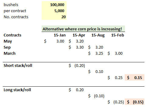
Hi @christoforou.n I moved to the error thread for the new GARP material. I agree with you: this should be stack/rolling LONG positions in futures contracts. The company is hedging a future purchase of corn, therefore wants a LONG hedge. This can be tested by substituting price increases into the exhibit: if we simulate price increases, then the stack/roll hedge needs to produce a net gain to hedge. Specifically, here is the given scenario in 8.20 such that the short stack/roll produced a gain (and the long produces a loss) of 0.15:

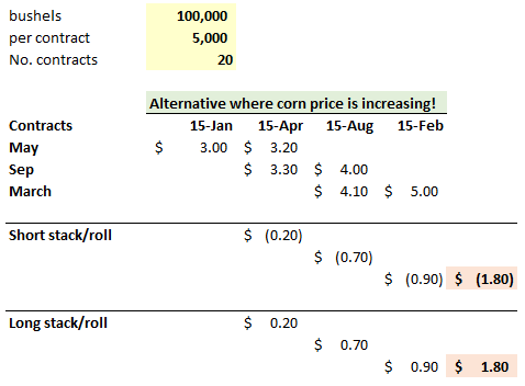
But below is an alternative scenario of rising corn prices. In order to hedge the purchase at higher prices, we need the LONG position stack/roll (lower panel) because we need a net profit--in this case $1.80--to offset the higher prices. (of course, a difference scenario would be prices dropping and the long stack/roll would produces losses, appropriate to the hedge). Thank you!

 

[bradnhopkins]

Two more from the Quantitative Analysis text:

Chapter 9, regression diagnostics- references in the end of chapter practice questions are made to the RESET test for specification and the Chow test, but those two tests are not discussed in the actual reading at all (I think the lack of reference to the RESET test is a gross over-sight since it is a tool available in most statistical packages).

This may be a question where I am just not seeing it, but question 10.18 specifies that we should forecast GDP using an AR(2) model, which at \[ Y_t \] where t=0 requires two values for the previous two time-steps, \[ Y_{t-1} \] and \[ Y_{t-2} \]. We are only given the value for \[ Y_{t-2} \], so I don't understand how GARP expects anyone to estimate the solution to this problem correctly. The solution has a value for \[ Y_{t-1} \] which the student cannot possibly be aware of, unless it was buried in a paragraph somewhere.

More generally, I feel that beginning with Chapter 8 there is a bit of a disconnect between the level and content of the readings and that of the practice questions which I feel could have been avoided with a better proof-reading and editing process.

 

[ruben169]

Hi David, others,

I spotted a mistake in the answer to question 12.20 in Book 4. The convexity calculations contain 2 mistakes in one equation: 1200.15 - 1199.85 = 0.3 (instead of 1200.15 - 1195.85 = 3).

Best, Ruben

 

[ruben169]

Hi all,

I have a question re practice question 13.17 in Book 4.

The question deals with interpolating par yield KR01s for a 7 year bond. The KR01 are 5 and 10 years.

As a result I would expect the 5 yr KR01 weight to be 2/5 and the 10yr KR01 to be 3/5, but the answer key contains exactly the opposite answer (without further explanation).

Could any explain to me whether this is correct and how they arrived this solution or it this (again) a mistake?

Best, Ruben

 

[mtakroosta]

Part I, Financial Markets and Products, Chapter 16, 16.11 last paragraph before summery, i.e. page 207:

To take a simple example, suppose that only two rates are offered in the market: a three-month rate and a five-year rate. Suppose further that both rates are 2.5% per year and that this reflects the market’s expectations (so that all expected future three-month rates are 2.5% per year). If the term structure of interest rates is flat at 2.5% (consistent with expectations theory), liquidity considerations will lead lenders to choose to commit funds for only three months, while borrowers will choose the five-year maturity. This will lead to a mismatch. As financial intermediaries try to match borrowers and lenders, market forces will lead to the five-year rates being pushed above 2.5%. For example, it might be found that making the five-year rate 3.5% (while keeping the three-month rate at 2.5%) will cause some borrowers to switch from five-month borrowing to three-month borrowing and some lenders to switch in the other direction. The end result is that supply and demand are matched at both maturities.

Apart from the fact that the text is obviously inconsistent, it makes more sense if we change all five-year words to five-month throughout the passage, and it seems that even the authors themselves meant so.

 

[mtakroosta]

Part I, Financial Markets and Products, Chapter 17, 17.8 the penultimate paragraph of the first column i.e. page 221:

The issuer default rate does not consider the size of the issues that defaulted, whereas the dollar default rate does. For example, suppose that there are 100 bonds with a total par value of USD 1 billion and that two bonds with a combined par value of USD 50 million default. The issuer default rate is 2% and the dol-lar default rate is 10%.

Should it not be 5% ???

 

[mtakroosta]

Part I, Financial Markets and Products, Chapter 19, 19.4. The first paragraph of the first column of page 250: Formula misnumbering.

April 15, 2019.12 First, the March 2020 Eurodollar futures can be used to estimate the 90-day forward rate for a 90-day period starting on March 16, 2020. This is assumed to apply to the 91-day period between March 16, 2020, and June 15, 2020, and Equation (19.2) (19.3) is used to estimate the zero rate for June 15, 2020. The June 2020 forward contract is then used to provide the forward rate for the 90-day period starting on June 15, 2020. This is assumed to apply to the 91-day period between June 15, 2020, and September 14, 2020, and Equation (19.2) is used to estimate the zero rate for September 14, 2020. This process is continued until the desired month is reached.

I also can not figure out the logic behind the equation of footpoint 12. If anyone could help me with it, it would be perfect.


Part I, Financial Markets and Products, Chapter 19, 19.5. The 4th paragraph of the first column of page 251: Formula misnumbering.

The three-month Eurodollar futures contract is designed so that a 1-basis point downward parallel shift in the yield curve gives rise to a gain of USD 25. This means that EF = 25. Equation (19.3) (19.4) gives the number of contracts required as:

 

[mtakroosta]

Part I, Financial Markets and Products, Chapter 19, Answer of Question 19.16. on page 255:

No coupons will be paid in the 31-day period between August 1 and September 1. The time to delivery is 31/365 = 0.0849 years. The dirty futures price is therefore:
132.5 e0.0849*0.04 = 132.9509

The accrued interest on September 1 is 5 * 61 123/184 = 3.3423. The clean futures price is therefore:
132.9509 - 3.3423 = 129.6086

Dividing by the conversion factor we obtain the estimated futures price as: 129.6086 1.2341
= 105.0227



* The 123 is the sum of (30+30+31+31+1)

 

[mtakroosta]

Part I, Financial Markets and Products, Chapter 20, Figure 20.5 on page 262:

The left box should be Company B A

 

[mtakroosta]

Part I, Financial Markets and Products, Chapter 20, Below table 20.3 on page 262:

If Company B borrows at the floating rate of 3.5% LIBOR + 0.9% indicated in Table 20.3, it has three sets of interest rate cash flows.
1. It pays Libor + 0.9%.
2. It pays X%.
3. It receives Libor.

 

[mtakroosta]

Part I, Financial Markets and Products, Chapter 20, 20.3. which is the last paragraph before 20.4. Page 263: Figure misaddressing.


Modifying the statement made in connection with Figure 20.2 20.7, we can say that the swap succeeds in exchanging a floating-rate liability for a fixed-rate liability if the company’s creditworthiness does not change so that it always borrows at the same spread above Libor.

 

[mtakroosta]

Part I, Financial Markets and Products, Chapter 20, The last paragraph of the second column i.e. Just above Figure 20.3. On Page 261.

The swap enables a ten-year three-year investment paying LIBOR minus 10-basis points to be exchanged for one paying 2.96%.

 

[dtammerz]

@David Harper CFA FRM
Part I, Financial Markets and Products (Book 3), Chapter 16 (Properties of Interest Rates) p. 203 regarding Dollar Duration and also Limitations of Duration: they seem to be referring to equation 16.4 (formula for continuous compounding) but should it be referring to 16.8 (relationship between duration and bond price)??




16.4

16.8

 

[David Harper CFA FRM]

Hi @dtammerz Thank you for noticing and sharing. I agree with you: it seems clear there reference should be to 16.8. Thank you. FYI, I haven't been keeping up this thread, there have turned out to be dozens of errors in the new material and I just haven't yet shared them back to this thread. There's been at least one or more error spotted each week this year, I'd say. After the exam, I'll begin the work of compiling the disparate observations. Thank you,

 

[dtammerz]

Hi @dtammerz Thank you for noticing and sharing. I agree with you: it seems clear there reference should be to 16.8. Thank you. FYI, I haven't been keeping up this thread, there have turned out to be dozens of errors in the new material and I just haven't yet shared them back to this thread. There's been at least one or more error spotted each week this year, I'd say. After the exam, I'll begin the work of compiling the disparate observations. Thank you,

@David Harper CFA FRM thank you very much for confirming that. I did not realize there were that many issues before finding this thread, but will be careful during my studies.

 

[MilaBank]

P1 Book 3 -Valuation and Risk Models 10th edition, chapter 9, p 131 :


The ask cash price is therefore USD 100.0733 (= 99.8281 + 0.2452). The cash amount received at maturity is USD 100.4375 (= 100 + (90.5 0.05* 0.875)). (May, 10/2019, p. 131)

May, B. (2019). 2020 Financial Risk Management Part I: Valuation and Risk Models, 10th Edition. [[VitalSource Bookshelf version]]. Retrieved from vbk://9780136594635

Hope it help anyone, cause i definitely wasted time trying to figure out why are they multiplying by 90.5 and not par 100