Problems in GARP's 2020 FRM material

[David Harper CFA FRM]

I will post here selected observations made (either by myself or subscribers/members) about the newest material. As most already know, the entire Part 1 FRM has experienced a big change, but the change can be deceiving in appearance because as I replied over on the reddit FRM board, with respect just to Part 1, the Part 1 learning objectives (LOs) are mostly unchanged. Rather, what changed is that GARP replaced the previous source material (an anthology of external authors) with their own internal content. However, most of the new GARP content maps directly (1:1) to previously assigned chapters. For this reason, the change appears big, but it actually small if your question is "In terms only of what I need to know for the exam, what is different in Part 1?" (Answer: not much is greatly different). Further, given this is GARP's first year, we should not expect anything near perfection in their material (put another way, it's GARP' first edition. The Hull chapters from last year, for example, had ten editions and many years of refinement/corrections).

For starters:

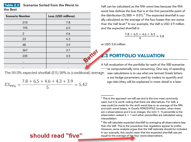
• [FRM-1 Foundations] The text reads "expected shortfall (ES), which is a statistical measure designed to quantify the mean risk in the tail of the distribution beyond the cut-off of the VaR measure." and EOC Question 1.25 reinforces as a TRUE statement that "ES is a statistical measure designed to quantify the mean risk in the tail of the distribution beyond the cut-off of the VaR measure." But this refers to the conditional VaR or tail conditional expectation (TCE) by confusing a quantile-threshold with a probability-threshold.
  • From my perspective, this should instead read something like (emphasis mine) "expected shortfall (ES), which is a statistical measure designed to quantify the mean risk in the tail of the distribution beyond the selected probability (or confidence) threshold"
  • Why does it matter? Because we know quantile-threshold definition causes confusion (for example) when confronting test questions. If the distribution is discrete, VaR is ambiguous. Here is a super-simple example: What is the 95.0% basic HS VaR when the super-tiny window is only n = 20 and given in L(+)/P(-) = {1, 2, 3, 4, 5, 6, 7, 8, 9, 10, 11, 12, 13, 14, 15, 16, 17, 18, 19, 20}. Strictly, the best answer is the (20*5%+1)th = 2nd worst loss, or 19. However, Jorion would say 20, and 19.5 is valid. Three fine answers (Excel will give you two more: there are probably fully five good answers!). That is, VaR is here ambiguous. If we define ES in terms of VaR (which is a quantile-threshold), then an ES defined in terms of the VaR is often also ambiguous. But we don't do that. We define ES in terms of probability-threshold, which is never ambiguous. If you think your ES has more than one answer, you are defining ES incorrectly. The 95% ES is the conditional mean: the weighted-average of the 5% (1 - 95%) loss tail. This forum has tons of discussion on this, and a more thorough explanation can be found on page 35 of Dowd's classic Measuring Market Risk (section 2.3.2).

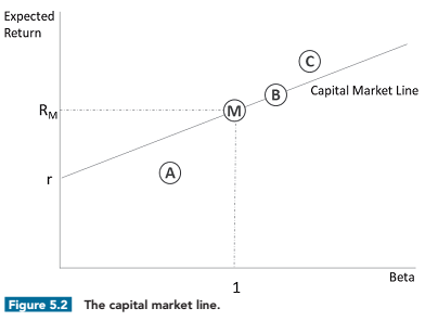
• [FRM-5 Foundations] The text goofs the CML saying, "Figure 5.2 shows the capital market line, defined as the linear relationship between the expected rate of return and systematic risk." However, is the security market line (SML) that plots return against beta; aka, systematic risk; the capital market line (CML) plots against standard deviation (aka, total risk, volatility). I have a video on this topic here https://forum.bionicturtle.com/thre...ne-cml-versus-security-market-line-sml.21443/
  
  
  

• [QA Chapter 8: Regression with Multiple Explanatory Variables] Credit to @jimmykaw who observes apparent typo on page 127, such that text probably should read:
  

  "As explained previously, adding an additional explanatory variable usually increases R2 (because it decreases RSS) and can never decrease it. On the other hand, including additional explanatory variables (i.e., increasing k) always increases ξ. The adjusted R2 captures the tradeoff between increasing ξ and decreasing RSS as one considers larger models. If a model with additional explanatory variables produces a negligible decrease in the RSS when compared to a base model, then the loss of a degree of freedom produces a smaller R2." -- 2020 Financial Risk Management Part I: Quantitative Analysis, 10th Edition. Pearson Learning Solutions, 10/2019

• [VRM-1 Learning objective] This is incorrect: "Describe spectral risk measures and explain how VaR and ES are special cases of spectral risk measures." Value at Risk (VaR) is not (a special case of) a spectral measure because it is a dirac delta function that violates the non-negativity weighting function requirement of a spectral. VaR and ES are special cases of the general risk measure; but only ES is spectral and coherent, but VaR is neither. Effectively the general risk measure is spectral if and only if (iif) it is coherent.
  As replacement, I proposed either of the following two correct statements:
  • "Describe spectral risk measures and explain how VaR and ES are special cases of the general risk measure." or also plausible:
  • "Describe spectral risk measures and explain how ES is spectral but VaR is not spectral (even as both are special cases of the general risk measure)."
    
    

 

[emilioalzamora1]

Hi @David Harper CFA FRM,

just wondering why the removed all the reference books/papers in the learning objectives? This makes it way more difficult for future candidates to look up topics in the appropriate books I suppose....

Are they going to publish their own book like the CAIA does?

 

[David Harper CFA FRM]

Hi @emilioalzamora1 I hope you are doing well! In Part 1, GARP did publish their own books. The learning objectives still do exist, now they are associated with GARP's chapters, although most of GARP's chapters map 1:1 to same external readings. Is that what you meant?

I'm not exactly sure what you mean by "why the removed all the reference books/papers in the learning objectives?". GARP still has LOs. The LOs are still associated with readings (albeit GARP chapters instead of external book chapters, for Part 1).

 

[emilioalzamora1]

Hi @David Harper CFA FRM

thanks for your reply! Yes, can't complain. Have been away from the forum for a while but as I am taking the PRM now I will be back more regularly I assume

The LOs are there as you said but the external book chapters/authors have been removed (they had reference books for all the sections in Part I and II) and this makes it much more difficult which "external books" candidates should consul for exam prep. I mean the VaR topic is discussed at a different level of detail in Dowd vs Choudhry for example. If you just have the plain LOs now, candidates may miss the level of detail/difficulty if they look up things in a source they may find appropriate instead of having the source/author given in the LOs.

 

[David Harper CFA FRM]

@emilioalzamora1 oh yes, I completely agree (i made similar point over at https://trtl.bz/2v3J591)

I don't know how this will play out. I just read the MPT/CAPM reading (Chapter 5) and it contains no illustrated examples of the performance measures (e.g., Sharpe) which is astounding (and it's just lightweight overall). The previous reading was sufficient, but this won't be sufficient/standalone for candidates. (Good for EPPs, I suppose, but ...?) Another example, in Topic 3, for many of the chapters John Hull is a (this is all just my opinion, it goes without saying!) better reference than the new chapters if only because Hull has more illustrated examples. GARP's chapters are shorter (as the OP notes on reddit, which is noted as an advantage), but my observation is that the efficiency is often due to fewer illustrated examples and simplifications. My specific example is Exotic Options: to me, you are better off referring to the Hull's Chapter (assigned in 2019 and prior) for depth on Exotic Options simply because, in my opinion, you need to see illustrated examples of exotics to understand exotics.

So when you say "candidates may miss the level of detail/difficulty," I could not agree more. This is the biggest issue and, given this is the first year, it remains to be seen how this aspect will be received. Not unrelated, GARPs EOC questions are not nearly exam-like, they are mostly true/false questions that are too superficial to prepare for the exam ... it's not enough to answer a superficial question like "15.5. List four types of compound options." ... it's almost the same point. EPPs may argue this is all a benefit to them and an opportunity for them to add value to customers. Thanks,

 

[David Harper CFA FRM]

In VRM-2 (Calculating and Applying VaR), I get two different values (see red circles below) when I recreate the 2.2 historical simulation.

 

[mukeshramawat]

Hi David,

Are changes (deletion, addition etc) in FRM 2 curriculum issued by GARP confirmed or there could be further updates ?

Thanks
Mukesh

 

[David Harper CFA FRM]

Hi @mukeshramawat As some errors have been observed, I think we can expect an errata at some point ...

 

[Nicole Seaman]

Hi David,

Are changes (deletion, addition etc) in FRM 2 curriculum issued by GARP confirmed or there could be further updates ?

Thanks
Mukesh

@mukeshramawat

I just wanted to add to David's above comment to say that if you referring to the actual syllabus in regard to the learning objectives that have been added/removed in 2020 (and not the errors in the GARP source books that are discussed in this thread), then those are confirmed and will not change. GARP has not stated anything about changing the actual syllabus or learning objectives after they released them in December. David's comment is in relation to GARP's source books, which contain errors that have been pointed out in this thread. I hope this helps!

Nicole

 

[David Harper CFA FRM]

In VRM-2, expected shortfall (ES) is defined in terms of what should instead be called tail conditional expectation (TCE) or conditional VaR. See below. I have reported to GARP this is problematic for three reasons:

1. It is inconsistent with the expected shortfall (ES) that is defined in Part 2 (per the Kevin Dowd assignment) which is a proper probability-delimited ES. Kevin Dowd's classic text has been the bible--and survived throngs of scrutiny by better people than me--on this (for the FRM) for over a decade.
   • There is an additional inconsistency: The P2 FRM (MR-1: Dowd Chapter 3) defines HS VaR as the [(1 - α)×N + 1]th ranked loss. According to this definition, in this dataset of 500 observations, the 99.0% VaR refers to the 1%*500 + 1 = 6th worst loss, which is 3.7. If we accept 3.7 as the VaR, then the quantile-delimited ES must be the average of the worst five losses! So even according to the P2 definition of VaR, the answer should be 5.42.
2. It is inconsistent with the last 10+ years of definition of ES in the FRM; e.g., it is inconsistent with presumably all EPP discrete-type ES questions
3. It enables multiple valid answers (not a desirable feature for a popular exam-type question)

Why does this matter?

I explained the first part of the problem (above) already. The most popular exam-type test of an ES is a basic HS ES. So let's take the example in GARP's Table 2.3 where, out of n = 500 sorted observations in L(+)/P(-) format, the worst seven losses are 7.8, 6.5, 4.6, 4.3, 3.9, 3.7, and 3.5. What is the 99.0% ES? The FRM has always followed Kevin Dowd's technical precision so that the answer is the conditional average of the 1.0% tail, an answer that is always unambiguous and never depends on the corresponding 99.0% VaR; in this case, the answer is 5.42, as shown below, because the 1.0% probability-delimited tail includes 5 observations (5/500 = 1.0%). If we allow ES to be the average of he losses "worst than the 99.0% VaR" then logically we must admit that the 99.0% VaR can be either 5.8 or 5.42 (or a midpoint) and then we must admit there are multiple ES answers. If the VaR is variant, than an ES that depends on VaR must also be variant. But we've always taught that ES is unambiguous. VaR is a quantile, but ES is a conditional probability-delimited average.

But now consider a different question about this same loss dataset: What is the 99.50% ES? If we use this "new" ES, then we first determine the 99.50% VaR is 4.6 (unlike the 99.0%, the 99.50% has only one VaR solution: it doesn't fall on a border but squarely in the middle of the third observation). Then, I would expect we would compute (7.8 + 6.5)/2 = 7.15 because these are the two "losses that are worse than the VaR." But, under this approach all of the ES from [99.40%, 99.60%] have the same value (!), yet we might expect the value to decrease slightly, we might expect 99.55% to be L/P greater than 99.45% ...

Compare to our proper probability-delimited ES which never gives more than one answer (a convenient feature for an exam!), the 99.50% ES is given by the conditional average of the worst 0.50% tail: (7.8 * 0.20% + 6.5 * 0.20% + 4.6 * 0.10%) / 0.50% = 6.64. This is how the FRM has always defined the ES, and still defines the ES in Part 2. Notice, further, that this ES does naturally decline as we increase confidence from 99.40% ES to 99.60% ES. (Always trust Kevin Dowd, his book has survived as a classic for a long time!).

In any case, at a minimum (obviously), if only for the sake of consistency with Part 2, the correct answer must be that either approach is acceptable. Although I really would prefer this approach in the text be called conditional VaR (or TCE) so that ES can maintain its elegant purity.

 

[David Harper CFA FRM]

In FRM-5 (Modern Portfolio Theory, MPT, and the Capital Asset Pricing Model. CAPM), only one version of the information ratio is defined (see below). I have reminded GARP that the FRM needs to allow for two definitions of the information ratio; this has been the case in the FRM since 2012. Specifically, the new new 2020 text (Chapter 5, see below) defines only the active IR; i.e., IR = excess_ return ÷ active_risk. However,

• In 2012, we pointed out that FRM-assigned authors Jorion/Bodie/Grinold implied different variations on the information ratio. I suggested the rule should be the principle of ratio consistency and ratio consistency allows for either an active IR or a residual IR. Helpfully, Question #3 in GARP's 2012 Practice Exam Part 1 was amended (see below) to clarify what has been the guidance ever since: "The information ratio may be calculated by either a comparison of the residual return to residual risk, or the excess return [dh note: i.e., active return] to tracking error [dh note: assume active risk, but clarification not needed in this case]."
  For that discussion see https://forum.bionicturtle.com/threads/information-ratio-definition.5554/
• Why does this matter? Because the more technical IR is the residual IR. If you run datasets, your are prone to correctly calculate alpha as the regression intercept. If you use this alpha (aka, residual return) and also enforce ratio consistency, your tracking error will be the residual version: IR = α/σ(α). In short, if you use a proper alpha and you enforce ratio consistency, residual IR is the correct version; active IR is more convenient because it is easier to calculate, is the trade-off.
• Here is another reason that the IR in Part 1 needs to be either residual/active: to be consistent with Part 2!
  • Assigned Andrew Ang clearly defines IR as a residual IR.
  • Also in Part 2, Bodie often defines IR as residual IR. See detailed discussion/interpretation of Bodie's alpha and tracking error here https://forum.bionicturtle.com/threads/unsystematic-risk-alpha.6993 and here https://forum.bionicturtle.com/threads/p2-t8-18-statistical-significance-of-alpha-bodie.5578
• Note on terminology where I will illustrate with an example: Rf = 3.0%, market portfolio's return = 9.0% (ie, market portfolio's excess return is 6.0%) and portfolio's beta, β(P,M) = 1.50. Although I'm using the CAPM to illustrate with the really simple single-factor case, keep in mind alpha/IR/TE are meant for more sophisticated multi-factor models:
  • Active return is the portfolio's return in excess of the benchmark. In my example, if the Portfolio returns 14.0%, then active return is 14.0% - 9.0% = +5.0%.
  • Residual return (aka, alpha) is the portfolio's return and and therefore adjusted by beta). In my example, alpha is 14.0% - 3.0% - (1.5 β * 6.0%) = +2.0%; we can might say alpha is the active return with respect to a risk-adjusted (beta-adjusted) benchmark, which can lead to the confusion. CAPM holds that expected (ex ante) alpha is zero; an ex post alpha is the regression's intercept
  • Tracking error does suffers ambiguity; it can refer either to active risk, σ(Rp - Rb; ie, active return), or it can refer to residual risk,σ(α = alpha).
    
    
    

 

[bradnhopkins]

Here is what I have found so far:

Book 1, Chapter 5: Question 5.4 does not follow logically from either prior questions or the readings. In equilibrium all assets will fall along the SML, and therefore take on some Beta value such that \[ \beta_i\in\mathbb{R} \]. There is insufficient information either in the question or in the text to conclude that the correct betas are -1, 0, and 2.

Book 2, Chapter 5 (page 65): The formula for Bias for the sample variance s^2 is Bias(s^2)= E[s^2] - σ^2 = σ^2/n per the text, but doing the actual math you wind up with Bias(s^2)= E[s^2] - σ^2 = -σ^2/n. I've checked the result in Wolfram Alpha's CAS engine, and it is indeed -σ^2/n. I cannot find a third party result confirming or disproving this on Google (I can only get as far as validating equation 5.7), and I would welcome anyone who can do so.

 

[Frodo81]

Here is what I have found so far:

Book 1, Chapter 5: Question 5.4 does not follow logically from either prior questions or the readings. In equilibrium all assets will fall along the SML, and therefore take on some Beta value such that \[ \beta_i\in\mathbb{R} \]. There is insufficient information either in the question or in the text to conclude that the correct betas are -1, 0, and 2.

Same for Q 5.5, right? Given the question, there is not a unique answer - or do I miss something?

 

[David Harper CFA FRM]

Hi @Frodo81 I agree with you, it's clear what they meant: Question 5.4 is incomplete and has no way to answer, but its answer is given as three betas: β(A) = -1.0, β(B) = 0, and β(C) = +2.0.

Then by itself Question 5.5 cannot be answered, but the intention was to build off (include) the same betas from Question 5.4, such that we can answer the question: "The riskless rate of interest is r = 5% and the market portfolio is characterized by E(RM) = 13% and sM = 15%. Assume three stocks have the following betas: β(A) = -1.0, β(B) = 0, and β(C) = +2.0. CAPM implies that the expected return of stocks A, B, and C are ..." Then we get ER(A) = 5.0% + (-1.0)*8.0% = -3.0%; ER(B) = 5.0% + (0)*8.0% = 5.0%; and ER(C) = 5.0% + 2.0*8.0% = +12.0%. Thanks!

 

[Hamam]

Hello,
Please see below. Is this correct when p is defined as 1 minus alpha?

"The confidence level, α, represents the probability that an event (e.g., daily loss) will be
less than (or equal to) the VaR quantile. Alternatively, the significance level, p,
represents the probability that a loss will be worse than the VaR"

 

[finhoe]

Hi @David Harper,

Would appreciate if you could check if the table 10.3 'Default Premium' is correctly printed in your opinion? The explanations make references to an AR(3) even though there isnt a \gamma_3 parameter on that table. The only \gamma_3 parameter i see is on the next table 'Real GPD Growth rate'. If im mistaken, would love if you could give a short explanation of that particular example?

 

[David Harper CFA FRM]

Hi @Hamam where are you reading that? (I cannot seem to find it in GARP's Part 1 material. This thread is focused on issues in GARP's materials). But to answer your question: yes, that is a fine way to describe VaR. Many people will naturally expect alpha, α, to be the significance level because by convention α is the probability of a type I error (see https://en.wikipedia.org/wiki/Type_I_and_type_II_errors), so they expect α to be the 0.1%, 1.0% or 5.0% (rather than the 99.9%, 99.0%, or 95.0%). However, we cannot get religious about the symbols (I think religions can take symbols seriously, but as an aspiring mathematician I don't think mathematical symbols can be religious!) The above is actually how Kevin Dowd defines VaR, he signifies the confidence level with α, and his significance level is 1 - α = p. (Is he your source?). So, if we do have α = 5.0% such that p = 95.0%, we can express VaR either as:

• The probability of experiencing a loss less than the VaR quantile is no more than 95.0%. Or my slight preference is the alternative:
• The probability of experiencing a loss greater than (aka, worse than) the VaR quantile is equal to 5.0% (or: is not more than 5.0%)

(why do I have a preference? Thank you for asking. It's subtle. The latter brings attention on VaR's feature that VaR, unlike ES, says nothing about the magnitude of the loss in excess of the quantile. The former, in a sense, focuses attention on the "known" body of the distribution, while the latter reminds us that the loss can be anything beyond the VaR. The two expressions above are mathematically equivalent, yet they draw attention to different aspects of the distribution and I prefer the expression that draws attention to the un-sized loss tail.)

@finhoe good question! I am not sure. I just forwarded your question to GARP. To be candid, I haven't analyzed GARP's new P1 Chapter 10 (time series). Let's get real for a moment: time series nowadays needs to be illustrated in a reproducible code workbook. In a code workbook, you'd be able to confirm by drilling down. How can anyone with exposure to time series actually learn it this way? I will update here when i get some feedback ...

 

[GarryB]

I have noticed an error in FRM CH 2 Question 2.14
QUOTE - 2.14 MGRM was exposed to a shift in the price curve from
backwardation to contango, which meant that the program
generated huge margin calls that became a severe
and unexpected cash drain.
A. True
B. False
UNQUOTE
The GARP book gives answer as B. - Can you please confirm the right answer.

 

[David Harper CFA FRM]

Thank you @GarryB good catch. This Q&A apparently wants to be "True" but there is an important caveat: it is a lazy, imprecise question. The MGRM case has been assigned since the start of the FRM so it has been extensively covered by several authors. Let us make a note of something: the shift in the forward curve (aka, futures price curve ... it is lazy to call it a "price curve") from contango to backwardation does not itself generate huge margin calls.

Consider (eg) a spot price of $40.00 and a long futures contract (ie., MGRM's hedge) under oil backwardation (the initial state) so that say the futures price is $32.00. Imagine a shift to contango without any change in the spot price; e.g., say futures price leaps up to $45.00 (i.e., contango). That's dramatic to illustrate, but this sort of futures price increase which would not itself create a margin call. Quite the opposite for a long, it would generate excess margin! The shift to contango per se did not create the margin calls.

Rather, in MGRM what created huge margin calls was the unexpected drop in oil spot prices (the shift to contango actually mitigates the margin calls) because this drove the drop in near-month futures contract prices (source: Allen Case Studies, previous FRM assignment).

The shift from backwardation to contango (as our members well know) implies a loss in the roll yield (aka, roll over return) for the long futures position. Losses due to roll over are different than margin calls! Of course, there was a third factor (accounting) such that:

1. Unanticipated drop in stop price drove drop in (highly correlated) near month futures prices (this was stack and roll, so they were short term contract) which caused huge margin calls
2. Shift from backwardation to contango created roll return losses
3. Accounting: MGRM would have been okay in the US because they could have shown net profits by booking unrealized forward contract gains (ie, forward sales to customers which which the underlying exposure that they where hedging). But under German rules, they long position short-term future contracts losses could not be (accountin-gwise) offset by the short position long-term forward contract gains. Many authors consider this the actual death knew because it was the huge reported losses that led to confidence run on MGRM. I hope that's interesting!

In summary, the following are TRUE statements::

• MGRM was exposed to a shift in the forward curve from backwardation to contango (aka, curve risk), the realization of which created roll return losses
• MGRM was also exposed to a drop in the spot price (and correlated near-month future prices) risk), the realization of which created margin calls.

So it does appear to be a typo, but when the typo is corrected, it masks a deeper flaw.

(If the question does intends to be false because the shift-to-contango did not per se cause margin calls, then it is still a poorly written question because it doesn't properly parse the cause and effect.)

 

[David Harper CFA FRM]

Foundations (Part 1), EOC Chapter 5, Question 5.10 (hat tip @DShim27 and @amit.m.sharma ). To the question "If σ(A) = 20% and σ(B) = 40% and a portfolio is formed with half the money invested in each stock then σ(P) must be" ... should have an answer of "between 10% and 30%" (which is not given). See https://forum.bionicturtle.com/threads/garp-2020-books-question-5-10.23107/#post-81072 ie..,

• sqrt[0.50^2*0.20^2 + 0.50^2*0.40^2 + *0.50*0.50*0.20*0.40*(-1.0)] = 10.0%
• sqrt[0.50^2*0.20^2 + 0.50^2*0.40^2 + 2*0.50*0.50*0.20*0.40*(+1.0)] = 30.0%