Errors Found in Study Materials P1.T2. Quantitative Methods (OLD thread)

[Nicole Seaman]

Please use this thread to let David and I know about any errors, missing/broken links, etc. that you find in the materials that are published in the study planner under P1.T2. Quantitative Methods. This will keep our forum much more organized. We appreciate your cooperation!

PLEASE NOTE: Our Practice Question sets already have links to their specific forum threads where you can post about any errors that you find. The new forum threads are for any other materials (notes, spreadsheets, videos,etc.) where you might find errors.

Information needed for us to correct errors:

• Reading
• Page number
• Error

 

[Kaiser]

Page 42 (Stock)

1. An increase in the or does not necessarily mean that an added variable is statistically significant.
2. A high or does not mean that the regressors are a true cause of the dependent variable.
3. A high or does not mean that there is no omitted variable bias.
4. A high or does not necessarily mean that you have the most appropriate set of regressors, nor does a low or necessarily mean that you have an inappropriate set of regressors."


I guess "or" means R-square.

Rgds,

 

[kevolution]

Hi,

As I was studying I noticed in the Stock & Watson Study Notes that you mentioned F-stat formula for homoskedastic to be ((SSRres - SSRunres) / q) / (SSRunres / n - kunres - 1) ..

however in one of the problems on the Study Guide it mentions that we can use R^2 in place of SSR, but on the denominator it does (1-R^2unres) / n - kunres - 1
which to me seems contradictory to the above formula? (Question & Answers #4)

Can you please clarify?

 

[Nicole Seaman]

@David Harper CFA FRM Can you confirm this is an error in the notes that needs to be fixed and let me know. Thanks!

Nicole

 

[kevolution]

Actually, I found my answer here:

https://forum.bionicturtle.com/threads/p1-t2-222-homoskedasticity-only-f-statistic.5480/

I think it would definitely be helpful to include the reversal equation with R^2 in the Study Notes!

 

[jacobweiss2305]

Hi All,

I was wondering if you could provide clarification on one of the formulas on your Diebold study notes.

On page 8, the it says SSR = MSE*T, and R^2 = 1 – SSR/TSS, R^2 = 1 – (MSE*T)/SSR  MSE = (1-R^2)*TSS*(1/T)

Why is R^2 = 1 – (MSE*T)/SSR and not R^2 = 1 – (MSE*T)/TSS? Shouldn't the denominator be TSS and not SSR?

I am sure I making a simple math mistake. Thanks in advance for the help!

Sincerely,
Jacob Weiss

Note from Nicole: This has been fixed in the pdf and updated in the study planner.

 

[David Harper CFA FRM]

Hi @jacobweiss2305 Yes, absolutely true. Sorry. Thank you! It should read: Because R^2 = 1 – SSR/TSS, R^2 = 1 – (MSE*T)/TSS --> MSE = (1-R^2)*TSS*(1/T). We will fix this ...

 

[SyroneDavid]

Hi friends, is it just me or should that last plus sign be an equal sign instead. so its E(et^2 | omegat-1) = E(et^2).
page 31 diebold chap 8 notes

 

[David Harper CFA FRM]

Hi @SyroneDavid Yes, for sure, it's our typo: the ε(t) is independent (zero-mean) white noise so it's conditional (squared) expectation equals its unconditional. Apologies from us, but super catch. Thank you!

 

[theapplecrispguy]

In the Stock & Watson Chapter 4 Notes on Univariate Linear Regression I have two questions:
1. On page 12 there is an example that uses a sample of 10 data points. The calculation of the standard deviations of X and Y and the covariance between X and Y all appear to use "n" as a divisor rather than "n-1". For a sample, is this an error or are both acceptable?
2. On page 16 in the example of student to teacher ratios and test scores there appears to be a disconnect between the data and the regression. The data would suggest that there is a positive correlation between the two variables (test scores increase as student teacher ratios increase) whereas the regression suggests a (more likely) negative correlation. I realize that the data is reproduced from the Stock and Watson reading. Am I missing something?
Thanks

 

[David Harper CFA FRM]

Hi @theapplecrispguy great observations (I gave you a star just because I appreciate attention to the details, that's why we are here!)

• You are right: especially if the sample is small like this (n = 10), the proper standard deviation would be a sample standard deviation that uses the (n-1) denominator; ie, a standard deviation based on an unbiased variance rather than an MLE variance. However, when the purpose is to calculate the correlation or beta (both of which are unitless), it will not matter because the (n) or (n-1) cancel. The note's correlation is actually based on population standard deviations, ρ = 0.7640 = 4.650 pop cov/(2.872 * 2.199 pop σs), but could have been equivalently calculated with samples because the total effect = [1/(n-1)]/(sqrt[1/(1-n)] * sqrt[1/(1-n)]) = 1.0 (cool!). In this case, with samples, ρ = 0.7640 = 5.1667/(3.02765*2.335). Beta is unitless correlation multiplied by cross-volatility (ratio of volatilities) such that similarly the (n-1)s cancel. In this case, the population-based beta, as shown in the notes, β = 0.7640*2.120/2.872 = 0.5636, but it's the same as the sample-based β = 0.7640 * 2.233582/3.02765 = 0.5636. You are right about the variances and standard deviations, they each have sample vs population variants; as does covariance, it's sometimes easy to forget that covariance generalizes the variance so it has sample variant. However, correlation and beta do not necessarily have a sample/population difference (Excel does not provide them, to my knowledge), although as usual, there are always alternative estimators, so they could have alternate estimators that are different (such estimators have never been in the FRM syllabus).
• The page 16 table (which mimics S&W table 4.1, although based on the actual source data, so it is true replication, as you can see in the learning XLS) is not making any pair-wise comparison between the two variables; eg, at the 10 percentile, the STR of 17.3 is a quantile (decile) of the univariate set of scores but it has no relationship to 630.4 which is the 10 percentile of the TestScore variable. Put another way you could not infer any actual pairs (STR, TestScore) from this exhibit which is a basic EDA/summary exhibit. I hope that's helpful!

 

[theapplecrispguy]

Hi @theapplecrispguy great observations (I gave you a star just because I appreciate attention to the details, that's why we are here!)

• You are right: especially if the sample is small like this (n = 10), the proper standard deviation would be a sample standard deviation that uses the (n-1) denominator; ie, a standard deviation based on an unbiased variance rather than an MLE variance. However, when the purpose is to calculate the correlation or beta (both of which are unitless), it will not matter because the (n) or (n-1) cancel. The note's correlation is actually based on population standard deviations, ρ = 0.7640 = 4.650 pop cov/(2.872 * 2.199 pop σs), but could have been equivalently calculated with samples because the total effect = [1/(n-1)]/(sqrt[1/(1-n)] * sqrt[1/(1-n)]) = 1.0 (cool!). In this case, with samples, ρ = 0.7640 = 5.1667/(3.02765*2.335). Beta is unitless correlation multiplied by cross-volatility (ratio of volatilities) such that similarly the (n-1)s cancel. In this case, the population-based beta, as shown in the notes, β = 0.7640*2.120/2.872 = 0.5636, but it's the same as the sample-based β = 0.7640 * 2.233582/3.02765 = 0.5636. You are right about the variances and standard deviations, they each have sample vs population variants; as does covariance, it's sometimes easy to forget that covariance generalizes the variance so it has sample variant. However, correlation and beta do not necessarily have a sample/population difference (Excel does not provide them, to my knowledge), although as usual, there are always alternative estimators, so they could have alternate estimators that are different (such estimators have never been in the FRM syllabus).
• The page 16 table (which mimics S&W table 4.1, although based on the actual source data, so it is true replication, as you can see in the learning XLS) is not making any pair-wise comparison between the two variables; eg, at the 10 percentile, the STR of 17.3 is a quantile (decile) of the univariate set of scores but it has no relationship to 630.4 which is the 10 percentile of the TestScore variable. Put another way you could not infer any actual pairs (STR, TestScore) from this exhibit which is a basic EDA/summary exhibit. I hope that's helpful!

Thank you. Clear explanations. I conclude that if the question (#1 above) had asked for the standard deviations I should give the sample standard deviations rather than the population standard deviations but that, as you note, it doesn't matter for beta and correlation.

Should the last sentence on page 12 of the notes which calculates the slope read: "Because the slope is equal to sigma(x,y)/sigma^2(x)=rho(x,y)*sigma(y)/sigma(x)"?

 

[David Harper CFA FRM]

Yes, great catch, that is a typo. It should read exactly as you show. The regression of Y on X entails β(Y, X) with respect to X so that σ^2(X) is the denominator. Thank you! (@Nicole Seaman I think we can wait until the next batch to include this, it is not quite worth uploading a new version; ie, non urgent)

 

[ziminli1228]

Hi,

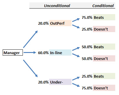
I am looking at R13.P1.T2.Miller study notes and need some help. On page 107, for the 80% non-star manager who are underperformer or just in-line performer, underperformer has the beat/doesn't of 25%/75% while in-line performers have the equal split of 30% vs. 30%. Could you please provide more color why the binomial tree is still giving 25%/75% for 80% non-star?

Thanks

 

[David Harper CFA FRM]

Hi @ziminli1228 Apologies but the binomial tree on p 107 is a mistake (also on p 108). I was already aware of this error and we have the fix coming; it should show the following to reflect the 3-stage problem:

 

[FlorenceCC]

Hi,

I was wondering if there was maybe an issue with the formulation of the sample problem #2 on page 101 of the Miller study notes (Bayesian analysis).
Question number asks "what is the probability that this manager is a star now?", but it does not define what "now" is - only after looking at the answer do we understand that this asks the probability the manager is a star now given he has beaten the market over the past three years (I think?)

 

[David Harper CFA FRM]

Hi @FlorenceCC As part of my youtube series, it happens to be that I recorded a video reviewing this problem (Miller Chapter 6 Sample #2), see below.

This sample question is perhaps not "exam-level" quality due to the slightly loose wording. I would not say it's wrong (is just my opinion) because I think it's right to infer that the second question is asking for the posterior (conditional) probability given the "evidence" of three years of beating the market:

"A new manager was added to your portfolio three years ago. Since then, the new manager has beaten the market every year. What was the probability that the manager was a star when the manager was first added to the portfolio? What is the probability that this manager is a star now? After observing the manager beat the market over the past three years, what is the probability that the manager will beat the market next year?"

... but, at the same time, to qualify as exam-level a good question should be precise and explicit. As somebody who write questions constantly, I agree with the spirit of your point: I would definitely want to edit that second question, because a good question does not hang people up in semantic interpretation like this question very well could. I hope you like my video about this question, thanks!

 

[ziminli1228]

In S&W chapter study notes, p36 where it denotes the k as number of slope coefficients. It says in the case for a two-variable regression, k=1. I think it was meant to say in a single-variable regression, k=1?

 

[David Harper CFA FRM]

Hi @ziminli1228 Right, very observant. It's actually a legacy from the prior assigned FRM reading, where the author called the regression given by Y = a + bX a two-variable regression because there is an independent variable (aka, regressor) and a dependent variable (aka, regressand). It has logic, in my opinion, when we think about the difference between variables and coefficients in the regression. But it's probably confusing under the S&W reading (assuming GARP doesn't switch this reading). I tend to call this a univariate regression (as opposed to multivariate), but on the other hand, the prior approach had (has) the virtue of specifying how many variables; e.g., a four-variable regression has three independent variables. We should probably purge instances of two-variable regression, as the syllabus seems to refer to this as a "single regression." Thanks!

 

[FlorenceCC]

Understood. Thank you!