You are using an out of date browser. It may not display this or other websites correctly.
You should upgrade or use an alternative browser.
You should upgrade or use an alternative browser.
Discount Rate and Growth rate...in commodities futures.
- Thread starter shivanin
- Start date
Hi @shivanin This recent post should be helpful https://forum.bionicturtle.com/threads/contango-backwardation-and-trading-cheap.10654/#post-51933
Although, in terms of the exam, you don't need to "go deep" on understanding this, you can (for the time being) go shallow. To go deep, if you want, you might examine my illustrated XLS, which is here (http://trtl.bz/1008-commodity-lease; caveat: I haven't published this yet as there remains at least one minor technical issue to resolve). The short answers are:
Hi @gargi.adhikari It's no problem, it's true the notation between authors is not consistent, but it's also true we probably can't understand all of this without understanding the notation. Sometimes, when I get stuck on the math, I find the best thing I can do is slow down, take a step backwards and re-read the more fundamental setup to a concept. In this case, as far as I am concerned F(0) is just an abbreviated form of F(0,T); Hull tends to use the former, and McDonald the latter. But they are always synonyms, in my experience. It is currently August, if I look at the corn futures prices (see http://www.cmegroup.com/trading/agricultural/grain-and-oilseed/corn.html) I see that the December 2017 contract has a recent price of $3.64 per bushel. As December is four months forward, we can represent this observed (aka, traded) price with: F(0, 4/12) = F(0, 0.33) = $3.64; i.e., we can enter the contract to buy corn in December and pay $3.64 in December, or we can promise to deliver corn in December and receive $3.64 in December. Imagine now stepping forward in time one month (ie, imagine we travel forward to September): this same contract's price, this contract for December delivery, will be signified by F(0, 3/12) = F(0, 0.25). If you haven't yet, I strongly encourage looking at http://www.cmegroup.com/trading/agricultural/grain-and-oilseed/corn.html ... we can see there is currently a futures corn curve: F(0, 1/12) = $3.51; F(0, 4/12) = 3.64; F(0, 8/12) = $3.77. All of these are currently observed (traded prices) which is the meaning of the '0' in F(0,T).
In regard to your cases:
- In Hull's cost of carry chapter and model, as the exploration is largely around a single future time interval, T, the use of F(0) is just an abbreviation of F(0,T).
- Re: "I had thought F0= to be the Futures Price Observed Today for Delivery at Time= 0= today:" this should be the spot price, S(0). As we approach maturity--ie., as (T) decreases in F(0,T)--we expect the futures price to converge to the spot price. But otherwise, we specifically do not expect F(0,T) to equal S(T). If (T) = 4 months or 0.33 years, then please notice, there is no currently observed such thing as S(0.33); i.e., we cannot currently observe the spot price of corn in December. But we can have an expected future spot price of corn in December, denoted E[S(t)] or E[S(T)]. But we only expect F(0) = E[S(t)] if r = k (ie., no systematic risk).
So please note, from the beginning of this thread, I have maintained there are three key variables really:
- Case A: F(0) = E[St]*exp[(r-k)T is correct and this is the perhaps more "theoretical" because it involves un-observable factors, namely E[S(t)] but also the discount factor (k) is not as observable as, say, the storage cost of corn.
- Case B: F0= S0* EXP[( Rf + Storage Costs ) - ( Div + Yield ) * T] is also correct as the COC model; I moved your "T" inside the square brackets.
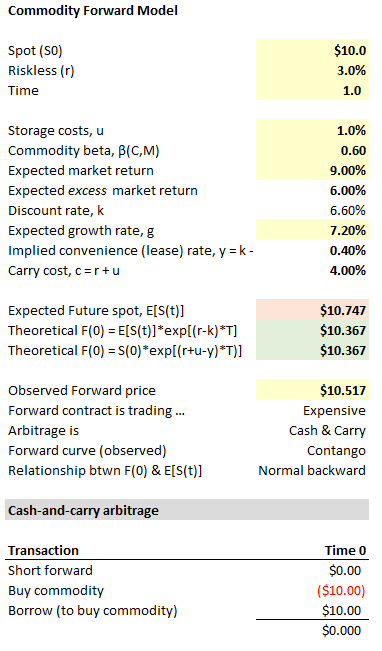
If you like, here is a draft of my commodity COC model (that will be in the next version of the massive Hull learning XLS, it builds on the current version in the Hull XLS): https://www.dropbox.com/s/590uw43t29ey0ap/0817-commodity-lease.xlsx?dl=0
- Theoretical F(0,T) which is given by the COC model
- Observed F(0,T) which is the traded price and, if it different than theoretical F(0,T), they we say it is "trading rich" or "trading cheap" (and this is a general idea: trading rich/cheap refers to an traded-observed price that doesn't match the model price, and is to be expected if for no other reason that the technical factors like supply/demand but also fundamental factors specifically, the model may be incomplete. Options can trade cheap/rich, bonds can trade cheap/rich. These are statements comparing a model output to an observed price).
- Expected future spot price, E[S(t] ... and, of course there is S(0)
... but this is only for intermediate/advanced viewing please: there are still some little kinks to address
... I show you just to show you how it contains (in green cells) two version of the theoretical F(0) per your two cases ($10.367 below) and how they must match. Also, this model outputs the typical scenario: Contango (because c > y) and Normal backwardation (because β > 0). I hope that's helpful!

Although, in terms of the exam, you don't need to "go deep" on understanding this, you can (for the time being) go shallow. To go deep, if you want, you might examine my illustrated XLS, which is here (http://trtl.bz/1008-commodity-lease; caveat: I haven't published this yet as there remains at least one minor technical issue to resolve). The short answers are:
- The theoretical forward price per the cost of carry model adds the risk-free rate, per all of the examples of course, and subtracts the convenience yield but the lease rate effectively substitutes for the convenience yield (both are benefits of ownership); i.e., Theoretical F(0) = S(0)*exp[(+r+u-y)*T)]
- Neither the discount rate nor the (expected) commodity growth rate appears directly in this COC model. However either can be indirectly referenced; e.g., Theoretical F(0) = E[S(t)]*exp[(r-k)*T], where (k) is the discount rate.
- The discount rate per CAPM is k = Rf + β(commodity, market factor)*ERP. How can we interpret it? In theory, current commodity spot price is the present of the total return to commodity ownership (including income and convenience/lease) discounted at the discount rate, which for a risky commodity (β>0) must be greater than the Rf rate.
- The growth rate is simply the expected growth rate in the spot price of the commodity. In my XLS, (k-g) = (y+u) which implies: if there is no storage (cost) and no convenience/lease, the growth rate will equal the discount rate. But a more typical scenario is that the discount rate differs from the expected (spot price) growth rate. If this part is confusing, my oft-used analogy is: a total stock return (TSR) includes both price appreciation (ΔS) and dividends (I) such that abstractly TSR = ΔS + I and so ΔS = TSR - I. When a stock pays dividends, we discount at the TSR but we expect the share price to grow less than the discount rate due to the dividend. Price growth is only one component of ownership.
- Lease rate as convenience yield is subtracted from the risk-free rate (it is a benefit of ownership). However, it can be negative when inferred from traded prices, as has been the case with the gold lease rate, but this is considered a surprising result and requires an even deeper dive on lease rate. I hope that's helpful!
Last edited:
Thanks a lot David for such good explanation.Hi @shivanin This recent post should be helpful https://forum.bionicturtle.com/threads/contango-backwardation-and-trading-cheap.10654/#post-51933
Although, in terms of the exam, you don't need to "go deep" on understanding this, you can (for the time being) go shallow. To go deep, if you want, you might examine my illustrated XLS, which is here (http://trtl.bz/1008-commodity-lease; caveat: I haven't published this yet as there remains at least one minor technical issue to resolve). The short answers are:
- The theoretical forward price per the cost of carry model adds the risk-free rate, per all of the examples of course, and subtracts the convenience yield but the lease rate effectively substitutes for the convenience yield (both are benefits of ownership); i.e., Theoretical F(0) = S(0)*exp[(+r+u-y)*T)]
- Neither the discount rate nor the (expected) commodity growth rate appears directly in this COC model. However either can be indirectly referenced; e.g., Theoretical F(0) = E[S(t)]*exp[(r-k)*T], where (k) is the discount rate.
- The discount rate per CAPM is k = Rf + β(commodity, market factor)*ERP. How can we interpret it? In theory, current commodity spot price is the present of the total return to commodity ownership (including income and convenience/lease) discounted at the discount rate, which for a risky commodity (β>0) must be greater than the Rf rate.
- The growth rate is simply the expected growth rate in the spot price of the commodity. In my XLS, (k-g) = (y+u) which implies: if there is no storage (cost) and no convenience/lease, the growth rate will equal the discount rate. But a more typical scenario is that the discount rate differs from the expected (spot price) growth rate. If this part is confusing, my oft-used analogy is: a total stock return (TSR) includes both price appreciation (ΔS) and dividends (I) such that abstractly TSR = ΔS + I and so ΔS = TSR - I. When a stock pays dividends, we discount at the TSR but we expect the share price to grow less than the discount rate due to the dividend. Price growth is only one component of ownership.
- Lease rate as convenience yield is subtracted from the risk-free rate (it is a benefit of ownership). However, it can be negative when inferred from traded prices, as has been the case with the gold lease rate, but this is considered a surprising result and requires an even deeper dive on lease rate. I hope that's helpful!
Hi David,
can I only have one of both: Lease rate or convenience yield in the exponent? Because if I lease it i can't take the advantage of the convenience yield?
Or do I have always to consider if exists: lease rate and convenience yield and storage cost?
1. r+u-lease-convenience
2. r+u-lease
And what do you mean with:
"the lease rate effectively substitutes for the convenience yield" and "Lease rate as convenience yield is subtracted"
Dies it mean: If I have both (lease rate and convenience yield) i only take the lease rate into account and ignore the convenience yield?
Thanks a lot
Hi @QuantFFM Right, I've struggled with this. I cannot make them both work simultaneously in the model, really. I discussed my most recent model is mentioned recently here at https://forum.bionicturtle.com/threads/contango-backwardation-and-trading-cheap.10654/#post-51933 and here is the XLS https://www.dropbox.com/s/590uw43t29ey0ap/0817-commodity-lease.xlsx?dl=0 (screenshot below). You will notice that I have one value for both of them (because I was not able to build an integrated view where they are both contributing separately).
Per my comments above, I basically view lease rate and convenience yield as synonyms in the cost of carry model: they are each the subtracted benefit of ownership that is less explicit than the explicit benefit of dividends or income. In the carry model, there are either costs or benefits of ownership, and they are explicit or implicit. My current view is that lease and convenience are synonymous because they are both implicit benefits of ownership, compared to dividends which are explicit (the dividend will be received, the lease rate may or may not be received depending on whether the asset is lent).
But consider McDonald's footnote #5 on page 174 (emphasis mine) ....
... my interpretation of McDonald (which of course might be wrong) is that I do not see him distinguishing in the quantitative model, especially in the following sense which is fundmental: being implicit benefits, either lease (or convenience) is inferred as the "plug variable" that is implied by the forward price (in other words, unlike storage costs where we have a hard estimate input, the convenience/yields are inferred from the traded price; they make the observed forward price match the COC model price). If that's true, then I'm satisfied to treat them as synonymous. In regard to his distinction, my hunch is that he really just means the convenience yield is a generalization of the lease rate. The lease rate is the option to lend. But the convenience yield is the broader, implicit benefit of ownership that may or may not include the option to lend (at the least rate). If that's accurate: lease rate implies convenience, but convenience does not necessarily imply lease rate (does not necessarily mean you can lend for profit, but rather your benefit is otherwise expressed). If this is true, then I think it justifies only a single "convenience yield" input, which embeds any/none lease rate. That's my thinking on it, I hope it's additive!

Per my comments above, I basically view lease rate and convenience yield as synonyms in the cost of carry model: they are each the subtracted benefit of ownership that is less explicit than the explicit benefit of dividends or income. In the carry model, there are either costs or benefits of ownership, and they are explicit or implicit. My current view is that lease and convenience are synonymous because they are both implicit benefits of ownership, compared to dividends which are explicit (the dividend will be received, the lease rate may or may not be received depending on whether the asset is lent).
But consider McDonald's footnote #5 on page 174 (emphasis mine) ....
"Convenience Yields: The discussion of commodities has so far ignored business reasons for holding commodities. For example, if you are a food producer for whom corn is an essential input, you will hold corn in inventory. If you hold too much corn, you can sell the excess. However, if you hold too little, you may run out of corn, halting production and idling workers and machines. The physical inventory of corn in this case has value: It provides insurance that you can keep producing in case there is a disruption in the supply of corn. In this situation, corn holdings provide an extra nonmonetary return called the convenience yield. [see footnote 5] You will be willing to store corn with a lower rate of return than if you did not earn the convenience yield. What are the implications of the convenience yield for the forward price?
Footnote 5. The term convenience yield is defined differently by different authors. Convenience yield generally means a return to physical ownership of the commodity. In practice it is sometimes used to mean what we call the lease rate. In this book, the two concepts are distinct, and commodities need not have a convenience yield. The lease rate of a commodity can be inferred from the forward price using equation (6.7).]"
... my interpretation of McDonald (which of course might be wrong) is that I do not see him distinguishing in the quantitative model, especially in the following sense which is fundmental: being implicit benefits, either lease (or convenience) is inferred as the "plug variable" that is implied by the forward price (in other words, unlike storage costs where we have a hard estimate input, the convenience/yields are inferred from the traded price; they make the observed forward price match the COC model price). If that's true, then I'm satisfied to treat them as synonymous. In regard to his distinction, my hunch is that he really just means the convenience yield is a generalization of the lease rate. The lease rate is the option to lend. But the convenience yield is the broader, implicit benefit of ownership that may or may not include the option to lend (at the least rate). If that's accurate: lease rate implies convenience, but convenience does not necessarily imply lease rate (does not necessarily mean you can lend for profit, but rather your benefit is otherwise expressed). If this is true, then I think it justifies only a single "convenience yield" input, which embeds any/none lease rate. That's my thinking on it, I hope it's additive!

Last edited:
Similar threads
- Replies
- 0
- Views
- 237
- Replies
- 0
- Views
- 198
- Replies
- 0
- Views
- 738
- Replies
- 0
- Views
- 809
- Replies
- 0
- Views
- 904

