Vasicek model recombining tree

[SalinaMiao]

Hi,

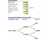
Can anyone demonstrate an example of how the rates in the Vasicek model tree is calculated? I am looking at Tuckman's chapter 9 study notes on page 57 (see attached). For example, how is the rate at (1,1) of 5.5060% calculated?

Thank you

 

[SalinaMiao]

also im not sure if its a typo? in the picture the formula says (k*theta-r) but at the top of chapter it says k*(theta-r). Which one is correct?

 

[David Harper CFA FRM]

HI @SalinaMiao The formula featured in the study note text is correct: dr = k (θ -r)dt + σdw. The displayed blue formula (that is part of the XLS screen) is incorrect (although the calculations are fine), apologies, and should match the text and consequently should appear as follows:

In regard to the calculations, they are in the XLS and explained by Tuckman in Chapter 7 (see below). However, the problem is that the node does not recombine naturally, see difference in values at node[2,1] inside red box:

Which he resolves as follows, I hope this explains(!):

 

[Rohit]

Hi @David Harper CFA FRM can we expect the calculation for r(uu) and r(dd) ? no where am I able to find a good explanation on the calculation. Thanks!

 

[nivethasridhar3]

HI @SalinaMiao The formula featured in the study note text is correct: dr = k (θ -r)dt + σdw. The displayed blue formula (that is part of the XLS screen) is incorrect (although the calculations are fine), apologies, and should match the text and consequently should appear as follows:

In regard to the calculations, they are in the XLS and explained by Tuckman in Chapter 7 (see below). However, the problem is that the node does not recombine naturally, see difference in values at node[2,1] inside red box:

Which he resolves as follows, I hope this explains(!):

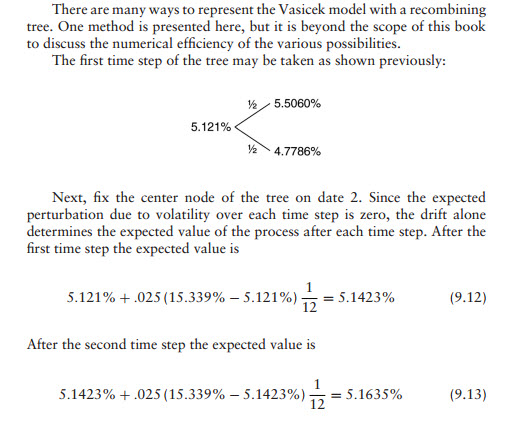
Hi, can you explain the sentence " The expected perturbation due to volatility over each time step is zero, the drift alone determines the expected value of the process after each time step". Why is that the case?

 

[David Harper CFA FRM]

Hi @nivethasridhar3 It is a good question because it relates to a key feature of these interest rate trees: they are not simulations themselves, nor are they they term structures, these binomial interest rate trees are "maps" that illustrate one sigma (standard deviation) jumps up and down. In the case of the Vasicek model, given by dr = k (θ -r)dt + σdw, this is a model of the movement in the short rate and it has two components: the deterministic drift, k(θ -r)dt, and the random shock (aka, stochastic) component, σdw. If we remove the stochastic component, then the tree would be a single (bending) line that bends from the current rate to the long-run mean, much like in GARCH(1,1), the prediction is a volatility that bends toward the long-run mean.

But the model contains a random shock, σdw. The binomial rate tree is a map of up/down jumps where σ = +/- 1.0. But the expected value (aka, mean) of this random normal variable is zero. The tree is showing how the rate looks if it jump up one or down one sigma, but the expected value is zero. That is the meaning of "Since the expected perturbation due to volatility over each time step is zero, the drift alone determines the expected value of the process after each time step". Good question, IMO, because it forces us to understand what this trees represent; over the years, I have noticed that many confuse them with a single simulation trial, or even the implied term structures (plots of the rate against maturity that are implied by the model). I hope that's helpful!

 

[Tonio57]

Hi David,

Thank you for all your answers. I'll go for the easiest example.

I still can't understand, when considering simple model 1: dr = s.dw with s annual volatility and dw normal random variable with variance t, why for the tree the upstate is r0 + s.srqt(1/12) and downstate is r0 + s.srqt(1/12)

Let's consider dw=0.25. I'd expect dr = s.dw and so r1 = r0 + s.0.25 or r1 = r0 - s.0.25 when applying the formula.
But in the answers everything is scaled while the formula states that annual vol. should be applied.

Then, how come the answer in that case will be r1 = r0 + s.0.25*sqrt(1/12) or r1 = r0 - s.0.25*sqrt(1/12)

In a nutshell, I don't get the link between dw and how trees are built up, when dw should be or not considered.... and if sqrt(1/12) factor is explained by scaling the annual volatility or explained by dw standard deviation.

Hope my question is clear.
Thanks in advance for your help!
Antoine

 

[David Harper CFA FRM]

Hi Antoine I'm not sure I follow you, sorry. In the simplest model (aka, model 1) we have dr = σ*dw where σ in an annual volatility and dw is a random normal with standard deviation of sqrt(Δt). The σ is really just an "untransformed" input. For example, if the annual basis point volatility assumption is σ = 1.60% but the steps are monthly, Δt = 1 /12, then what really matters is the periodic (per step) volatility (per SRR) is 1.60%*sqrt(1/12) = 0.4619%. The tree maps each monthly step, up and down not the full 1.60%, but the full periodic (monthly) volatility. And the simulation randomizes it. This post is hopefully helpful at https://forum.bionicturtle.com/thre...dw-by-sqrt-1-12-every-month.13745/#post-59068 i.e., new emphasis below in blue

Hi @QuantFFM dw is how Tuckman specifies the models; he scales the random standard normal rather than scaling the annual basis point volatility input (which would be more intuitive to me, too!). But I'm not sure it matters because the essential random shock is the product of three variables:

[random normal Z = N^(-1)(random p)] * σ[annual basis point volatility] * sqrt(Δt/12_months); i.e.,

• Random normal Z: a random standard normal, by definition µ = 0, σ = 1.0
• The annual basis point volatility; e.g., 1.60% or 160 basis points per annum. As usual, inputs should be in per annum terms
• Scaling factor per the usual square root rule (SRR) that assumes i.i.d. Notice I elaborated the full SRR to sqrt(Δt/12_months) because the denominator is whatever are the time dimension of the volatility input, in the case and as usual, per annum = 12 months. So to your second point, of course the 1-year volatility input can be scaled to monthly with 1.60% * SQRT(1 month/12 months) when our tree step is one month (i.e., numerator) and our input volatility is 12 months (i.e., denominator). Because we can assume this re-scaled monthly volatility is normal, it randomized by multiplying by a random normal Z.

It's just the case that models are specified by (random normal Z) * σ[annual basis point volatility] * sqrt(Δt) = [(random normal Z) *sqrt(Δt)] * σ[annual basis point volatility] = dw * σ[annual basis point volatility], so that dw is not random standard normal but instead a random normal, with standard deviation of sqrt(Δt), that scales (i.e., is a multiplier on) the annual basis point volatility. To me it's not different than itemizing all three with Z*σ*sqrt(Δt), and if he gains an advantage by using (dw) I don't really know what it is?! To your point, I don't know why his is better than: (random normal Z) * σ[annual basis point volatility] * sqrt(Δt) = (random normal Z) *[sqrt(Δt) * σ(annual basis point volatility)] = Z * σ[t-period basis point volatility]

I hope that's helpful, have a good week yourself!