VaR not Subadditive , Coherent Risk Measure

Is VaR Subadditive?


  • Total voters
    8
  • Poll closed .

Yash $$$

New Member
Hello, can anyone please explain the following?

How is VaR NOT subadditive?

To calculate portfolio VaR, we would use Portfolio mean & Portfolio standard deviation (which includes effect of correlation between each individual security in the portfolio), thus when we calculate Portfolio VaR it would always be equal or less than the aggregate VaR of each individual security in the portfolio, which satisfies the subadditivity criteria.

Also, please explain coherent risk measure (in simple terms)

if we slice the whole return distribution (where as in ES we slice only the tail portion) and weight each quartile according to risk aversion, how does this help in analysing the riskiness of a portfolio or security. and how is it better than VaR or ES.

Thank you.
 

ShaktiRathore

Well-Known Member
Subscriber
Hi there,
WE calculate the Var in the conventional way assuming the elliptical distributions like normal, lognormal etc. for the portfolio. The correlation used is also used for measuring the linear relationship between the variables not the non linear relationship which can exist and can distort the actual relationship or correlation. Considering non-elliptical distribution and non linear relationship (which reflects the reality) the Aggregate Var for the portfolio can be greater than the sum of VaR of each individual security in the portfolio. The theoretical framework hardly represents reality but this is the case.
Coherent risk measure is one which satisfies the following properties:
1. sub-additivity
2. monotonicity
3. cash invariance
4. homogeneity
for more details visit:
http://www.portfolioprobe.com/2013/01/14/the-incoherence-of-risk-coherence/
http://forum.bionicturtle.com/threads/the-incoherence-of-risk-coherence.6646/#post-22421

thanks
 

Yash $$$

New Member
Thanks again for the explanation, shakti.

For coherent risk measure calculation, (Chapter 3 Dowd)
they say...
"under ES estimation, the tail region is divided into equal probability sliced and then multiplied by the corresponding quantiles. under the more general coherent risk measure, the entire distribution is divided into equal probability slices weighted by the more general risk aversion (weighting) function"
so its more like a weighted average of values at different quantiles of the whole distribution (Rather than just the tail of the distribution)

so how is it a risk measure, when its focus is not on the tail of the distribution?

Also, one of the EOC question is.."Which of the following statements about expected shortfall estimates and coherent risk measures are true?"
to which the answer is "B.-- Expected shortfall and coherent risk measure estimate quantiles for the tail region"

So, i find the part in the notes and the answer of the question quite contradictory,
can you explain which one is actually right

Appreciate your help!!!

Yash
 

ShaktiRathore

Well-Known Member
Subscriber
Hi
Under ES estimation the tail region is assigned a distribution(e.g. extreme value or POT) now this distribution is divided into equal probability slices weighted by the more general risk aversion (weighting) function. The focus is on tail region only the difference is that the tail region itself follows a distribution which is then treated as said above to estimate the ES.

thanks
 

ShaktiRathore

Well-Known Member
Subscriber
Hi,
try this link also:http://forum.bionicturtle.com/threads/var-and-es-vs-sub-additive-measures.449/
The ES follow sub-additive property because as returns of X and Y are non elliptical then their simultaneous returns are also non elliptical but now we are taking average of those Vars and this averages of Vars approximates a normal distribution for large value of n, This is analogous to CLT that we takes variable with non normal distribution but sample of means follow a normal distribution for the observations hence we say that ES approximates a normal or elliptical distribution for large value of observations thus its bound to be sub-additive. Even if Vars are non elliptical their averages follow a normal distribution which is nothing but ES, ES in my opinion is both theoretically as well as practically well justified and is considered as more appropriate measure for measuring risk because it follows all properties of coherence while Var does not seems a viable candidate but still is used due to its simplicity and elegance. Overall ES is far more superior on theoretical grounds.

Take for example recent financial crisis which had a contagion effect on all the constituents of the portfolio. Thus is i hold A: 100$, std Dev=6% and B: 100$, std Dev=8% correlation between them as -.5 the portfolio has a std dev of sqrt(6^2+8^2-2*6*8*.5)=sqrt(52)~7.2%.This implies Var of 1.65*7.2%*200=39.2 at a CL of 95% thus we expect maximum loss not to exceed at 95% CL but during contagion effect all the constituents move in same adverse movement and they returns from them do not follow elliptical distribution. While calculating Var we assumed normal distributions of returns but during adverse situations the returns follow non elliptical distribution we need to come out with a special formula to calculate Var.During the crisis the returns are -50% leading to losses of 100$ which is far excess of Var predicted by us assuming normal distribution. Non sub-additive property does not hold because the actual losses exceeds the predicted losses.


hope it helps
thanks
 

filip313

New Member
Subscriber
Hello,

Here there is a really good explanation of why VaR does not satisfy the sub-additivity condition of coherent risk measures:
http://www.risk.net/risk-magazine/technical-paper/1506669/var-versus-expected-shortfall
(If the page does not load try to stop the loading and then refresh it).

The only problem is that I do not understand how VaR is calculated in the first example (when only 1 loan is considered).
I can see that the calculation is 1%/1.25% = 80% and that 80% for a uniform distribution is equal to a VaR of $2M, but I haven't been able to explain this formula using the classic conditional probability formulas.
Why do I need to divide 1% by 1.25%? I understand that 1% is because of the level of confidence of the VaR, but where does this formula come from?

Can someone please explain the caulculations step by step?

I think this is a great example and it would be really good to have a complete understanding of it.


Many Thanks
 

David Harper CFA FRM

David Harper CFA FRM
Subscriber
Hi @filip313 The article's example is very good. The unconditional loss distribution is:
  • most of the distribution: $200K profit
  • up to 98.750%: $200K profit
  • at 99.00%: $2 mm
  • at 99.25%: $4 mm
  • at 99.50%: $6 mm
  • at 99.75%: $ 8 mm
  • at 100.0%: $10.0 mm (I am "rendering" this "as if" it's discrete but it's continuous, these are just selected points)
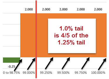
I think of this as a rectangle in the tail: height of $2.0 million and width of 1.25% (i.e., 99.75% t0 100.0%). We want the worst 1%. Because it's a rectangle, the worst 1% is (4/5) or (1%/1.25%) of the $10.0 mm. I hope that's helpful!

please note the excel labels are not aligned quite right but hopefully this helps:

100615-var.png
 
Last edited:

filip313

New Member
Subscriber
Hi @filip313 The article's example is very good. The unconditional loss distribution is:
  • most of the distribution: $200K profit
  • up to 98.750%: $200K profit
  • at 99.00%: $2 mm
  • at 99.25%: $4 mm
  • at 99.50%: $6 mm
  • at 99.75%: $ 8 mm
  • at 100.0%: $10.0 mm (I am "rendering" this "as if" it's discrete but it's continuous, these are just selected points)
I think of this as a rectangle in the tail: height of $2.0 million and width of 1.25% (i.e., 99.75% t0 100.0%). We want the worst 1%. Because it's a rectangle, the worst 1% is (4/5) or (1%/1.25%) of the $10.0 mm. I hope that's helpful!

please note the excel labels are not aligned quite right but hopefully this helps:

100615-var.png

Thank you David.

I think I understand, but can we solve this using the conditional probability formula?
i.e. P(A|B) = P(AB) / P(B)
where P(B) = 0.0125 and P(A|B) = 0.01
Or this does not make sense?
 

David Harper CFA FRM

David Harper CFA FRM
Subscriber
Hi @filip313 I think maybe it can be viewed as P(default)*P(Loss > $200K | default) = P(default, Loss > $200K); i.e., 1.25%*80% = 1.0% ... but personally, for myself, it's not easier to find the answer this way because the answer depends on understanding how we would use the uniform distribution within the 1.25% tail. Put another way, because it's a uniform (conditional) distribution, we know to multiply the 1.25% by 80% to retrieve the 1.0% that we are seeking. But the tail distribution might not be uniform, in which case the 1.0% VaR would not lie at (80% * 1.25%). To me, the key here is to understand:
  1. We seek the unconditional 1.0% quantile; i.e., the loss at which the area in the tail represents a 1.0% unconditional probability
  2. Given the 1.25% default region happens to be uniform (losses) in this case, where in region can be locate the 1.0% unconditional? Answer: because it's uniform, the unconditional 1.0% is located at 80% = 1.0%/1.25%.
So, a (visual or mathematical) understanding of the distribution is my personal preference, but I could be missing an easier way. Thanks,
 
Last edited:

David Harper CFA FRM

David Harper CFA FRM
Subscriber
Also, we forgot to mention the expected shortfall (ES) for this example, it's just a good example I think!

To re-cap the article's example: If a single $10.00 million loan has a 1.25% probability of default (PD) and its loss given default (LGD) is a uniform distribution with all recoveries from 0% to 100% being equally likely, what are (i) the 99.0% VaR and (ii) the 99.0% expected shortfall. What if instead we have a portfolio that holds two of these loans, but they are independent of each other?
 
Top