VaR and ES

[Kavita.bhangdia]

HI David,

1. If I have two portfolios : P1 with ES = ES1 at 95% confidance interval and P2 with ES = ES2 at 99% confidance interval.

How do we calculate the total Expected shortfall for the two portfolios.. Shall we convert 99% ES2 to 95% ( divide by 2.33 and multiply by 1.645) and add to 95% ES? Will they be linearly added? What if we have a correlation between the two portfolios?

2. I know Jorion says that while calculating VaR we should always take the absolute value of the portfolio ( irrespective of whether we are long or short).

If I have two portfolios
a) portfolio of long equities VaR1 and
b) portfolio of short equities VaR2

Then my total VaR should be VaR1-VaR2 because they are negatively correlated.. ( assume perfect negative correlation)
Am I correct?

Thanks,
Kavita

 

[David Harper CFA FRM]

Hi @Kavita.bhangdia

1. Great question, and instructive, but large scope depending on assumptions. Let's just address the question under your implicit assumption that both portfolios are normally distributed (and further that we are referring to a relative VaR so that scaling is easy; or, if you like, that drift is risk free and we are present valuing the VaR). In this case, ES aggregates for two normal portfolios in a manner similar to how VaR aggregates, as you suggest but with the following key difference: we aren't rescaling the VaR, we are rescaling the ES. So we would not use *1.645/2.33 but rather their ES analogs: standard normal 95% ES = NORM.S.DIST(NORM.S.INV(95%),FALSE)/(1-95%) = 2.062713 and standard normal 99% ES =NORM.S.DIST(NORM.S.INV(99%),FALSE)/(1-99%) = 2.665214. So to convert 99% to 95%, we would multiply by 2.063/2.665. For example, say P1 95% ES = 3.0 and P2 99% ES = 5.0, then

• if the P1 and P2 are perfectly correlated, the 95% ES of (P1+P2) = 3.0 + (5.0 * 2.063/2.665) = 6.87
  
• if the P1 and P2 are independent, the 95% ES of (P1+P2) = sqrt[3.0^2 + (5.0 * 2.063/2.665)^2] = 4.90; i assume you see the analogy to normal VaR?
• I will leave the correlated case for the upcoming Week in Risk (my newsletter this weekend), I think it's a good question, but it's not hard if you are following me so far

2. If they are normal with perfect negative correlation, then yes per VaR(p)= sqrt[VaR1^2 + VaR2^2 + 2*VaR1*VaR2*ρ] --> then when ρ=-1.0, VaR(p) = sqrt[VaR1^2 + VaR2^2 - 2*VaR1*VaR2] = VaR1 - VaR2. I hope that helps!

 

[Stuti]

Hi @David Harper CFA FRM - I wanted to know if we have a spreadsheet to calculate the Order Statistics Estimates of Standard Normal 95% VARs and the associated Confidence Intervals. I wanted to understand the calculations.

 

[Ashok_Kothavle]

Hello Mr David,

You have defined above

standard normal 95% ES = NORM.S.DIST(NORM.S.INV(95%),FALSE)/(1-95%) = 2.062713

This is for Standard Normal Variate. I was just wondering if instead of SNV, if I consider the Normal distribution with mean = 100 (say) and Stdev = 20, how will the expected shortfall be related the ES value obtained for SNV = 2.062713?

I tried,

NORM.DIST(NORM.INV(95%, 100, 20), 100, 20, FALSE)/(1-95%).

The Value I am getting is
0.10313564 which is obviously wrong. The value should be around 141.253730.

Incidently, if we consider the part of ES expression for SNV i.e. NORM.S.DIST(NORM.S.INV(95%),FALSE), the value obtained is 0.01313564 same as the answer I am getting for the complete expression for ES if I consider the Normal distribution with mean = 100 and Stdev = 20.

Not able to figure out where am I committing the mistake? It is my gut feeling that we should be able to establish some relationship with ES(for SNV) with ES(with some mean and stdev).

If we define

ES (with mean = 100, stdev = 20) = Mean + ES(w.r.t SNV) * Stdev
i.e. 100 + 2.062713 * 20 = 141.2542562 which is much closer to the value 141.253730.

This way, I guess we can calculate the expected shortfall for any Normal variate with non zero mean and non unitary standard deviation.

Can you guide?

Regards

 

[David Harper CFA FRM]

Hi @Ashok_Kothavle I do not know how to modify the standard normal ES given by the Excel function, as I understand that to be (by definition) a standard normal function. Given the location-scale invariance property of the normal, it seems like the easiest thing to do (per your second example) is simply re-located and scale the standard deviate. Notice Hull uses this approach:

That show's Hull's alternative approach to ES, but it nevertheless (in Excel) produces a standard normal deviate; for example, in your scenario of µ = 100 and σ = 20:

• 95% standard normal ES = EXP(-(NORM.S.INV(0.950)^2)/2) / (SQRT(2*PI())*0.05) = 2.063 standard deviate, such that 95% ES given µ of 100 and σ of 20 = 100 + 20*2.063 = 141.2543; equivalently
• 95% normal ES = 100 + 20 * NORM.S.DIST(NORM.S.INV(0.950),FALSE)/0.05 = 141.253

So, perhaps there is a way to tweak the "inside" of the second expression, but if so I just don't know that method (sorry), but on the other hand, it's not like we need to. Thanks!

 

[Ashok_Kothavle]

Dear Mr David,

Thanks a lot for this very very informative and prompt reply. Helped a lot to clarify few basic things.

Regards

Ashok

 

[Hassan2016]

Hi all. How can I calculate the ES using the excel?

I am already having a VaR model, Do I need to make some changes to calculate the ES?

 

[emilioalzamora1]

Hi @Hassan2016,

I will come up with a detailed explanation about several options you can choose from when calculating ES in Excel. This is always a great exercise for me as well to remind me of the concepts. Thanks for asking this type of question.

Remember that we are interested in the left-hand tail of the distribution. Hence we use the significance level (alpha) for the NORMSINV-function; the right-tail would require NORMSINV(1-alpha).

Expected Shortfall (ES) is the average of the worst 100 (1-alpha)% of losses in the tail.

There are two approaches:
1.) Variance-covariance
2.) Historical Simulation
(beyond the one - which is perhaps more tedious - given above by David with Excel's PI () function for 'pi')

1.) Variance-covariance (assuming 99% confidence level which then implies alpha = 0.01) under the assumption of zero mean and variance 1 (standard normal assumption):

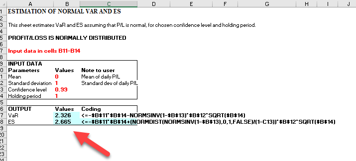
The formula is: NORMDIST[NORMSINV(0.01),0,1,0] / 0.01

which should yield 2.665%

1.1) Variance-covariance (assuming 99% confidence level which then implies alpha = 0.01) having a mean of 0.01% and a standard deviaiton of 1.6%

Then the above formula extends to:

- mu + ( NORMDIST[NORMSINV(0.01),0,1,0] / 0.01 ) * sigma
- 0.01% + [ ( NORMDIST[NORMSINV(0.01),0,1,0] / 0.01 ) * 1.6% ]

which should yield 4.25%

1.1.1) In case you have a certain wealth (portfolio value), V, invested and want to have the $(dollar) ES, we would simply have:

V * ( - mu + ( NORMDIST[NORMSINV(0.01),0,1,0] / 0.01 ) * sigma )

1.1.2) Alternatively one sometimes see the following formula where 'p' stands for the confidence level which yields the same result.

- mu + [ (1/(1-P) * (( NORMDIST[NORMSINV(0.01),0,1,0] / 0.01 ) * sigma) ]

2. Historical Simulation

We use Excel's AVERAGEIF-function (& = amerpsand in Excel!) here having (notice the 'minus' sign in front of the function! and the minus sign in front of the VaR!)

-AVERAGEIF(A1:A50, "<"&-VaR) + mu

where A1:A50 is your return row (this is just example) and where VaR denotes the Value-at-Risk calculated using Excel's Percentile function (notice the 'minus' sign in front of the function!)

-PERCENTILE(B1:B50, 1-confidence level) * sigma

where B1:B50 are your standardized returns which are: (your simple return for each period - mean)/sigma

[again, B1:B50 is a hypothetical assumption where your standardized returns in Excel may be calculated]

Please do also make sure you practice the following VaR conversions for the exam (hypotehtical figures!), they are tested all the time:

10-day 95% Var = 26
1-day 95% Var = 26/sqrt(10) = 8.22

10-day 95% Var = 26
1-day 99% Var = 26/sqrt(10) *ABS(2.33/1.64) = 11.65

1-day 99% Var = 35
1-day 99% Var = 35 * ABS(1.64/2.33)

For further explanations about ES please see one of the following sources:

1. Jon Danielsson, 'Financial Risk Forecasting'
2. Frank Fabozzi, 'Portfolio Construction and Analytics'

 

[Hassan2016]

Hi @emilioalzamora1

Thanks for reply, where can I find this explanation?

 

[emilioalzamora1]

give me some time please!

 

[Hassan2016]

@emilioalzamora1
Can I have this on an excel sheet? I can deliver you historical data

 

[emilioalzamora1]

I will not distribute any spreadsheets to single persons. If there are some further questions to the theory, please ask them here in the forum.

In case you are in dire need of some spreadsheets about VaR etc. I do recommend the following which comes with a full bunch of spreadsheets:

Simon Beninnga, 'Financial Modelling'

 

[Hassan2016]

Thank you @emilioalzamora1 will apply and revert if any.

 

[David Harper CFA FRM]

Hi @Hassan2016 Here is Kevin Dowd's normal ES spreadsheet https://www.dropbox.com/s/dgjys1yqdn60p7a/Normal ES.xls?dl=0 It should be consistent with @emilioalzamora1 's "1.1 Variance-Covariance" approach discussed above; keep in mind that, as discussed further up, that standard normal ES can be re-scaled with mean and variance (see Dowd's example 12.10 above). Dowd's ES spreadsheet is from his FRM-assigned book Market Risk http://amzn.to/2npoV11 Thanks!

 

[Hassan2016]

thanks @David Harper CFA FRM
it is very useful, if i need to replace 99% confidence level VaR by 99% confidence level ES, I will multiply by 2.665 instead of 2.33 correct?

 

[David Harper CFA FRM]

Hi @Hassan2016 Yes, exactly! (see below, i wouldn't know myself except by looking at the spreadsheet as these aren't familiar deviates ....) I assume you realize this is the 99% ES for a standard normal distribution, the XLS lets you change the µ and variance, σ^2, to re-scale to any normal 99% ES, so you just want to be mindful that most realistic distributions are not normal. This is another case of using the normal to illustrate. Thanks!