You are using an out of date browser. It may not display this or other websites correctly.
You should upgrade or use an alternative browser.
You should upgrade or use an alternative browser.
T4.ch1.pg14: VaR trend with holding period
- Thread starter Jaskarn
- Start date
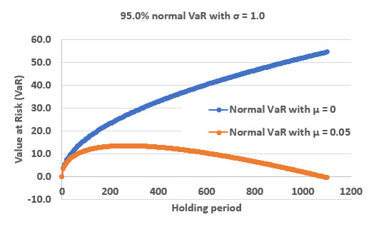
Hi @jaskaran Happy New Year, to you also!  The proper VaR is called an absolute VaR and is given by (Dowd's): aVaR = -Δt*μ + sqrt(Δt)*σ*z(α). This is the so-called normal VaR (i.e., arithmetic returns are normally distributed) rather than the "lognormal VaR," so this is our most common version of VaR in the FRM. I like to negate the drift but you can see this is the same as subtracting the drift: aVaR = sqrt(Δt)*σ*z(α) - Δt*μ. My plot assumes volatility, σ = 1.0. And in this example, the confidence level is 95.0%, so the normal quantile (aka, deviate) of course is z(α) = 1.645.
if we assume μ = 0, then:
10-day VaR = -Δt*0 + sqrt(Δt)*σ*z(α) = sqrt(10)*1.0*1.645 = 5.201
100-day VaR = -Δt*0 + sqrt(Δt)*σ*z(α) = sqrt(100)*1.0*1.645 = 16.449
250-day VaR = sqrt(250)*1.0*1.645 = 26.007
But if we assume μ = 0.050, then:
10-day VaR = -Δt*0 + sqrt(Δt)*σ*z(α) = -10*0.050 + sqrt(10)*1.0*1.645 = 4.701
100-day VaR = -Δt*0 + sqrt(Δt)*σ*z(α) = -100*0.050 + sqrt(100)*1.0*1.645 = 11.449
250-day VaR = sqrt(250)*1.0*1.645 = -250*0.050 + sqrt(250)*1.0*1.645 = 13.507
Absolute VaR is a return-adjusted risk measure (as opposed to risk-adjusted return measures like Sharpe or Treynor): The worst expected loss is mitigated (reducted) by the expected return (aka, drift) which is an expected profit in the case of market risk. Put another way, absolute VaR is the worst expected loss relative to the initial (today's) position because it "gives credit" for any expected gain/profit that would offset/mitigate the loss (the loss that is a function of volatility). So there is not a "skewness concept" here, and the normal distribution (i.e., of arithmetic returns) is assumed throughout. Rather, the difference is merely between no drift (μ = 0) and some drift (μ = 0.050). Hopefully, you can see also why, if the drift is zero--that is, if μ = 0, then absolutely VaR is equivalent to relative VaR. I hope that's helpful,
 The proper VaR is called an absolute VaR and is given by (Dowd's): aVaR = -Δt*μ + sqrt(Δt)*σ*z(α). This is the so-called normal VaR (i.e., arithmetic returns are normally distributed) rather than the "lognormal VaR," so this is our most common version of VaR in the FRM. I like to negate the drift but you can see this is the same as subtracting the drift: aVaR = sqrt(Δt)*σ*z(α) - Δt*μ. My plot assumes volatility, σ = 1.0. And in this example, the confidence level is 95.0%, so the normal quantile (aka, deviate) of course is z(α) = 1.645.
if we assume μ = 0, then:
10-day VaR = -Δt*0 + sqrt(Δt)*σ*z(α) = sqrt(10)*1.0*1.645 = 5.201
100-day VaR = -Δt*0 + sqrt(Δt)*σ*z(α) = sqrt(100)*1.0*1.645 = 16.449
250-day VaR = sqrt(250)*1.0*1.645 = 26.007
But if we assume μ = 0.050, then:
10-day VaR = -Δt*0 + sqrt(Δt)*σ*z(α) = -10*0.050 + sqrt(10)*1.0*1.645 = 4.701
100-day VaR = -Δt*0 + sqrt(Δt)*σ*z(α) = -100*0.050 + sqrt(100)*1.0*1.645 = 11.449
250-day VaR = sqrt(250)*1.0*1.645 = -250*0.050 + sqrt(250)*1.0*1.645 = 13.507
Absolute VaR is a return-adjusted risk measure (as opposed to risk-adjusted return measures like Sharpe or Treynor): The worst expected loss is mitigated (reducted) by the expected return (aka, drift) which is an expected profit in the case of market risk. Put another way, absolute VaR is the worst expected loss relative to the initial (today's) position because it "gives credit" for any expected gain/profit that would offset/mitigate the loss (the loss that is a function of volatility). So there is not a "skewness concept" here, and the normal distribution (i.e., of arithmetic returns) is assumed throughout. Rather, the difference is merely between no drift (μ = 0) and some drift (μ = 0.050). Hopefully, you can see also why, if the drift is zero--that is, if μ = 0, then absolutely VaR is equivalent to relative VaR. I hope that's helpful,
@Jaskarn
Think about it this way.
μ is your arithmetic expected return. If it is 0.05, then on average you're making 5% per year. Think of this as steady income you make regardless of the volatility. So over time, this becomes a larger and larger buffer against very bad outcomes. Over a long enough time period, the "build up" of 5% returns year after year will be greater than even the 95th percentile bad outcome, and the curve will start bending downwards. (assumes iid etc)
That's a terrific, intuitive explanation @ktrathen ! See below. I extended the same plot with the same simples assumptions (i.e., σ = 1.0 for but comparing zero drift in blue to μ = 0.050 in orange) and you can see how the VaR actually "breaks evens" at about 1,082 days because that's where μ*Δt = σ*1.65*sqrt(Δt). I hope that's helpful color adding to @ktrathen's point, thanks,


Similar threads
- Replies
- 0
- Views
- 261
- Replies
- 0
- Views
- 795
- Replies
- 0
- Views
- 1K
- Replies
- 3
- Views
- 1K
- Replies
- 0
- Views
- 1K

