T2 - Chapter 10 Stationary Time Series Notes

[Jaskarn]

Hi @David Harper CFA FRM

I am not able to understand below context. kindly help

Updated by Nicole to note that this is regarding the study notes in T2 - Chapter 10 Stationary Time Series on page 13.

As shown in the moving average process building equation above, the lagged shocks feed positively into the current value of the series, with a coefficient value of 0.4 and 0.95 in both the cases. It would be an obvious & false assumption that θ= 0.95 would induce much more persistence than θ= 0.4. It is a false assumption because the structure of the above MA(1) process accounts only for the first lag of the shock, leading to a short-lived memory usage in process building and the value of coefficient really does not have substantial impact on the dynamics of the process.

 

[David Harper CFA FRM]

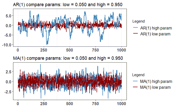
Hi @Jaskarn See image below where I simulate each of AR(1) and MA(1) with a low param versus a high param; in this case, my low param is 0.050 and my high param is 0.950. Notice how the AR(1) with high param exhibits "persistence" (in blue) versus the low param AR(1). However, in the case of the MA(1), it's hard to even tell the difference. The point is that you might expect an MA(1) with a weight of 0.95 to be more persistent than an MA(1) with weight of only 0.050, but it is not the case because an MA is only giving the weight to the last random white noise shock. I hope that's interesting.

My code at github: TBA

 

[Jaskarn]

Wow, thanks David that is very interesting.

 

[David Harper CFA FRM]

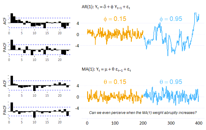
Indeed, I was having fun with the comparison so I ended up making some enhancements (which I will incorporate into a future version of the study notes). See below. In this revision, instead of overlapping the series, I simply use a single series but switch the weight in the middle (at 100 steps out of 200). I think this comparison is a better. I added the ACF and PACF because I discovered the wonderful patchwork package that lets you design multiple plots onto a single canvas. I shared this on LinkedIn.

Code is here https://github.com/bionicturtle/frm/blob/master/ma_vs_ar_v2.Rmd

 

[Jaskarn]

I think standalone MA(1) regression may not very useful for practical analysis. That's why we came up with ARMA models.

 

[ktrathen]

David, I have a related question. What is meant by "process invertibility" in this context?

 

[David Harper CFA FRM]

HI @ktrathen We use invertible functions a lot in the FRM, in particular the CDF probability function N(z) = p which "inverts" such that z = N^1(p). In the AR/MA time series context, invertability enables the translation of an MA(1) into an infinite AR(∞) series and similarly an AR(1) into an infinite MA(∞) series. Why would we want to invert an MA into an AR process? Because MA weights previous errors which are not obviously part of the observed series, the observed series is the set of observations and the AR process weights the observations. But this is not GARP's focus in Chapter 10 where invertibility is discussed. Rather, GARP's focus is the technical requirement that underlies the inversion of an MA into an AR or vice-versa: invertibility refers to when the lag polynomial has a multiplicative inverse: a(L)*a(L)^(-1) = 1; i.e., https://en.wikipedia.org/wiki/Multiplicative_inverse

Do we care about this invertibility? In a direct sense, not really. But we do care greatly about covariance-stationary, we basically want our models to be stationary and notice GARP's says "While it is not necessary to manually invert a lag polynomial, the concept of invertibility is useful for two reasons. First, an AR process is only covariance-stationary if its lag polynomial is invertible." That's why we care; the MA is always stationary (although you'll see there is a note about the advisability of selecting MA parameters such that the MA is invertible), but a sloppy AR might not be stationary and we much prefer a stationary process. In the Appendix to Chapter 10, the invertibility test is illustrated. Specifically, the roots of the lag polynomial's characteristic equation must lie with the unit circle.

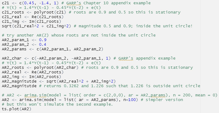
For the technically inclined, below is some of my code showing two models. First, I followed GARP's example in the Appendix, AR(2) given by Y(t) = 1.4*Y(t-1) - 0.45*Y(t-2) + ε(t) whose characteristic has roots of 0.9 and 0.5 (i.e., inside the unit circle) and so we can simulate this AR(2) model with arima.sim(). In the second case, I assumed AR params (i.e., 0.9 and 0.4) where the roots are not both inside the unit circle and R rejects the simulation with an error message "AR part of model is not stationary". I hope that's interesting!

 

[ktrathen]

Thanks David. I wish I had the time to dig into this a bit deeper. Pretty cool.