Risk free debt, merton model

[Kavita.bhangdia]

Hi David,

I was reading the Stulz chapter from GARP readings and what I understand is that in the PD calculation in Merton model, Stulz uses Risk free Debt ( F*exp(-r*t)) in the formulae

so instead of ln(asset value/face value of debt), he uses ln(asset value/present value of debt).

My understanding could be incorrect though.. Please can you help me clarify this.

Thanks,
Kavita

 

[ShaktiRathore]

Hi,
i think he just rearranges the formula:
According to merton model:
PD=N(-d2)
d2=(LN[V(0)/F(T)] + [mu - sigma^2/2]*T)/[sigma*SQRT(T)]
=>d2=(LN[V(0)*exp(-r*T)/F(T)*exp(-r*T)] + [mu - sigma^2/2]*T)/[sigma*SQRT(T)]
=>d2=(LN[V(0)/F(T)*exp(-r*T)] +LN(exp(-r*T)) + [mu - sigma^2/2]*T)/[sigma*SQRT(T)]
=>d2=(LN[V(0)/F(T)*exp(-r*T)] -r*T + [mu - sigma^2/2]*T)/[sigma*SQRT(T)]
=>d2=(LN[V(0)/F(T)*exp(-r*T)] + [mu -r+ sigma^2/2]*T)/[sigma*SQRT(T)] is the stulz's version where present value of debt F(T)*exp(-r*T) instead of face value of debt F(T) in the denominator.
thanks

 

[David Harper CFA FRM]

Hi @Kavita.bhangdia Actually Stulz does not use the risk-free rate in computing PD per the Merton model. For full background, see my note at https://forum.bionicturtle.com/threads/merton-model-a-summary-of-the-issues.5646/

But really briefly, Merton has two steps

1. Using call option pricing (ie., equity as call option on the firm's assets) in order to retrieve the the firm's asset (debt + equity) value and asset volatility, which does use the risk-free rate and does discount debt at the risk-free rate (consistent with BSM risk-neutral valuation), then
2. Estimates PD using the firm's asset return (not the risk free rate) and projecting a future distance to default. There is no present valuing with this step, nor any risk free rate involved. Step 1 is derivative valuation (which looks for an expected discounted value and assumes a risk-neutral distribution), but Step 2 is risk measurement which looks to the distribution of future values and the actual (aka, physical) distribution. Thanks,

 

[Stuti]

Hi

I have a question when evaluating the deb claim . The reading says : "Since equity is a call option on firm value, it is a portfolio consisting of delta units of firm value plus a short position in the risk - free asset. How did we arrive at this?

 

[Mkaim]

It's a little vague, but the closest I can come to this is through put-call parity. Put + Stock = Call + Risk-Free Bond (PV) --> P + S = C + B --> Solving for the call price you get C = P + S - B where -B is the short position in the risk-asset (or bond). I believe they mean "Put + Stock" as the delta units partly because the delta of the put is associated with the movement in the stock price of the firm.

 

[Stuti]

I tried using the Put call parity equation as well but could not arrive at the result. @David Harper CFA FRM - Can you explain this?

 

[David Harper CFA FRM]

Hi @Stuti and @Mkaim

This is the basic building block of BSM. There is more than one way to think about it. Hull builds from the one-step binomial model, showing that a riskless portfolio consists of a short call in one option plus Δ shares of stock. Using that idea, let (F) be the face value of the firm's debt which is analogous to the option's strike price, and ΔA = delta units of firm value which is analogous to delta units of stock value then:
risk-free payoff --> F(t) = Δ*A(t) - c(t), such that equity as call option c(t) = Δ*A(t) - F(t)
i.e., in the dynamic hedge a risk-free return is guaranteed if we continuously rebalance by hedging the short call, -c(t), with the purchase (i.e., hedge) of Δ units of the underlying asset, + Δ*A(t). This is just keeping the portfolio delta neutral (see Hull Ch 18 for scenario illustrations).

It may seems like equity as a call option on firm assets should be just, A(t) - F(t), without the delta, but consider this is more accurate in the M2M valuation. To illustrate. Say the firm's face value of debt is 80.00, due in two years, while its current asset value is $100.00. Assume Δ = N(d1) = 0.80; i.e., above 0.5 due to in the money. Currently, if the asset value increases by $10.00, the option value does not increase by the full $10.00, the increase is nearer to 10*N(d1) = $8.00. Long a full unit of asset against a written call would be an overhedge.

The other key is the dynamic of delta as the option (equity as call on assets) approaches expiration. Importantly, if it is in the money, Δ approaches 1.0 and if it is out of the money it approaches zero! So at expiration:

• If ITM (i.e., assets > debt) as maturity --> 0, then Δ --> 1.0 and c(t) = 1.0*A(t) - F(t) = A(t) - F(t) <-- as we expect at expiration, intrinsic value!
  
• If OTM (i.e., assets < debt) as maturity --> 0, then Δ --> zero and c(t) = 0*A(t) - F(t) = -F(t); ie, only obligation, worthless equity. Actually, true to the math, this is zero as in the dynamic rebalancing, while Δ --> 0, the net borrowing also approaches zero (note Hull's dynamic hedge is covered under the ITM scenario but is naked under the OTM scenario). I hope that helps!

 

[Stuti]

It's a little vague, but the closest I can come to this is through put-call parity. Put + Stock = Call + Risk-Free Bond (PV) --> P + S = C + B --> Solving for the call price you get C = P + S - B where -B is the short position in the risk-asset (or bond). I believe they mean "Put + Stock" as the delta units partly because the delta of the put is associated with the movement in the stock price of the firm.

Thanks David. This clarifies the question.

 

[Stuti]

hi @David HarperFA FRM

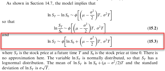
I was reading the merton in detail and am stuck at the following equation where log asset values follows a normal distribution with the following parameters:

 

[brian.field]

What is your question? I might be able to offer so thoughts.

 

[Stuti]

What is your question? I might be able to offer so thoughts.

I understand that in merton model we assume that the asset follows a log normal distribution, but i am unable to understand the mean term in the equation I have highlighted in red

 

[Mkaim]

I understand that in merton model we assume that the asset follows a log normal distribution, but i am unable to understand the mean term in the equation I have highlighted in red

The link below will tell you all you need to know about the Merton Model for the exam + more.

https://forum.bionicturtle.com/threads/merton-model-a-summary-of-the-issues.5646/

 

[David Harper CFA FRM]

Thank you @Mkaim

@Stuti The note to which Mkaim refers is my comprehensive effort. I would just add here that you will note that your formula is identical to Hull's 15.3, see below, which is the GBM process that informs the Black-Scholes (albeit, as I explain in the note, the key difference is that the Merton PD employs the asset's expected return, µ, whereas the BSM employs the risk-free rate, r, for the drift.):

 

[Stuti]

I understand that in merton model we assume that the asset follows a log normal distribution, but i am unable to understand the mean term in the equation I have highlighted in red

Thank you!

 

[Stuti]

The link below will tell you all you need to know about the Merton Model for the exam + more.

https://forum.bionicturtle.com/threads/merton-model-a-summary-of-the-issues.5646/

Thank you!

 

[Stuti]

Thank you @Mkaim

@Stuti The note to which Mkaim refers is my comprehensive effort. I would just add here that you will note that your formula is identical to Hull's 15.3, see below, which is the GBM process that informs the Black-Scholes (albeit, as I explain in the note, the key difference is that the Merton PD employs the asset's expected return, µ, whereas the BSM employs the risk-free rate, r, for the drift.):

Hi @David Harper CFA FRM ,

Can you also help me explain this concept. What does rolling down the curve mean? and when does it happen?

The benchmark for this corporate bond at issuance was the 10-year on-the-run Treasury with 5% coupon and maturity date August 15, 2011. As the bond has rolled down the curve, the current benchmark is the five-year on-the-run Treasury, which has a 3% coupon and matures on February 15, 2009. It has a yield-to-maturity of 3.037%. As the yield of the Ford bond is 5.94% and that of the benchmark is 3.04%, the yield spread is 290bp.

 

[Mkaim]

Hi @David Harper CFA FRM ,

Can you also help me explain this concept. What does rolling down the curve mean? and when does it happen?

The benchmark for this corporate bond at issuance was the 10-year on-the-run Treasury with 5% coupon and maturity date August 15, 2011. As the bond has rolled down the curve, the current benchmark is the five-year on-the-run Treasury, which has a 3% coupon and matures on February 15, 2009. It has a yield-to-maturity of 3.037%. As the yield of the Ford bond is 5.94% and that of the benchmark is 3.04%, the yield spread is 290bp.

Roll down typically means seasoning --> I am assuming the text is referring to the Maturity curve-->the bond is getting closer to its maturity as it ages, so its life (or WAL) is shrinking. For comparison purposes you want a Treasury bond with similar current life as your bond. In this case, there could be 5 years worth of seasoning (benchmark changing from 10 to 5 year Treasury).

 

[David Harper CFA FRM]

Hi @Stuti It would be helpful if you started a new thread (or attached to a relevant thread) when changing the topic. @Mkaim is symbolically correct about roll-down, but Tuckman gives a very technical (i.e., specific) definition. In chapter 3, he parses a bond's total price change (appreciation) into three components: (i) carry-roll-down, (ii) rate change and (iii) spread change. Carry-roll-down can be observed by the effect on bond price if the term structure used to discount the cash flows are unchanged (i.e., if rate change and spread are held constant). If the term structure is upward-sloping then, as @Mkaim implies, seasoning (i.e., just moving forward in time), will apply lower discount rates to the same cash flow; for example, initially the final cash flow for a 10-year bond will discount at the 10-year rate, but after one year, this same terminal cash flow discounts at a lower rate (lower because the term structure is upward sloping). This component, by itself, is the roll-down. Thanks,