Fran
Administrator
AIM: Describe credit factor models and evaluate an example of a single-factor model.
Questions:
304.1. Malz gives us a single-factor credit risk model, where a(T) is the log asset return. This single-factor model is sum of systemic risk contribution plus an idiosyncratic risk contribution:
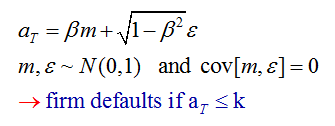
(Source: Allan Malz, Financial Risk Management: Models, History, and Institutions (Hoboken, NJ: John Wiley & Sons, 2011))
If a firm's systemic risk contributes 70% to its total risk (i.e., idiosyncratic risk therefore contributes 30%) and if the firm's unconditional default probability is 2.0%, what are the implied beta and (k) parameters?
a. beta = 0.56, k = -3.18
b. beta = 0.84, k = -2.05
c. beta = 1.07, k = -1.26
d. beta = 2.39, k = +1.11
304.2. Under Malz's single-factor credit model, a(T) = beta*m + SQRT(1-beta^2)*epsilon, a firm has a beta of 0.40 and an unconditional default probability of 3.0%. If we enter a modest economic downturn, such that the value of (m) = -1.0, what is the (downturn) conditional default probability?
a. 3.0%
b. 4.6%
c. 5.3%
d. 6.8%
304.3. Each of the following is an assumption, or implication of assumption(s), in Malz's single-factor credit risk model EXCEPT which is not?
a. (m) and epsilon (e) are standard normal variates; i.e., zero mean and unit variance
b. Because cov[m,e] = 0, a(t) is also a standard normal variate
c. Beta is related, but not identical to, a firm's equity beta: it captures the co-movement with an unobservable index of MARKET conditions, not with an observable STOCK index
d. The model conditions by changing epsilon, the "single factor," which necessarily increases the standard deviation of the default distribution
(Source: Allan Malz, Financial Risk Management: Models, History, and Institutions (Hoboken, NJ: John Wiley & Sons, 2011))
Answers:
Questions:
304.1. Malz gives us a single-factor credit risk model, where a(T) is the log asset return. This single-factor model is sum of systemic risk contribution plus an idiosyncratic risk contribution:
(Source: Allan Malz, Financial Risk Management: Models, History, and Institutions (Hoboken, NJ: John Wiley & Sons, 2011))
If a firm's systemic risk contributes 70% to its total risk (i.e., idiosyncratic risk therefore contributes 30%) and if the firm's unconditional default probability is 2.0%, what are the implied beta and (k) parameters?
a. beta = 0.56, k = -3.18
b. beta = 0.84, k = -2.05
c. beta = 1.07, k = -1.26
d. beta = 2.39, k = +1.11
304.2. Under Malz's single-factor credit model, a(T) = beta*m + SQRT(1-beta^2)*epsilon, a firm has a beta of 0.40 and an unconditional default probability of 3.0%. If we enter a modest economic downturn, such that the value of (m) = -1.0, what is the (downturn) conditional default probability?
a. 3.0%
b. 4.6%
c. 5.3%
d. 6.8%
304.3. Each of the following is an assumption, or implication of assumption(s), in Malz's single-factor credit risk model EXCEPT which is not?
a. (m) and epsilon (e) are standard normal variates; i.e., zero mean and unit variance
b. Because cov[m,e] = 0, a(t) is also a standard normal variate
c. Beta is related, but not identical to, a firm's equity beta: it captures the co-movement with an unobservable index of MARKET conditions, not with an observable STOCK index
d. The model conditions by changing epsilon, the "single factor," which necessarily increases the standard deviation of the default distribution
(Source: Allan Malz, Financial Risk Management: Models, History, and Institutions (Hoboken, NJ: John Wiley & Sons, 2011))
Answers:
") because we know that beta is correlation multiplied by cross-volatility.
because we know that beta is correlation multiplied by cross-volatility.