P2.T6.304. Single-factor credit risk model

Fran

Administrator
AIM: Describe credit factor models and evaluate an example of a single-factor model.

Questions:

304.1. Malz gives us a single-factor credit risk model, where a(T) is the log asset return. This single-factor model is sum of systemic risk contribution plus an idiosyncratic risk contribution:
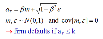
T6.304.1_formulas.png

(Source: Allan Malz, Financial Risk Management: Models, History, and Institutions (Hoboken, NJ: John Wiley & Sons, 2011))

If a firm's systemic risk contributes 70% to its total risk (i.e., idiosyncratic risk therefore contributes 30%) and if the firm's unconditional default probability is 2.0%, what are the implied beta and (k) parameters?

a. beta = 0.56, k = -3.18
b. beta = 0.84, k = -2.05
c. beta = 1.07, k = -1.26
d. beta = 2.39, k = +1.11


304.2. Under Malz's single-factor credit model, a(T) = beta*m + SQRT(1-beta^2)*epsilon, a firm has a beta of 0.40 and an unconditional default probability of 3.0%. If we enter a modest economic downturn, such that the value of (m) = -1.0, what is the (downturn) conditional default probability?

a. 3.0%
b. 4.6%
c. 5.3%
d. 6.8%


304.3. Each of the following is an assumption, or implication of assumption(s), in Malz's single-factor credit risk model EXCEPT which is not?

a. (m) and epsilon (e) are standard normal variates; i.e., zero mean and unit variance
b. Because cov[m,e] = 0, a(t) is also a standard normal variate
c. Beta is related, but not identical to, a firm's equity beta: it captures the co-movement with an unobservable index of MARKET conditions, not with an observable STOCK index
d. The model conditions by changing epsilon, the "single factor," which necessarily increases the standard deviation of the default distribution

(Source: Allan Malz, Financial Risk Management: Models, History, and Institutions (Hoboken, NJ: John Wiley & Sons, 2011))

Answers:
 

ashanks

New Member
Hi BT community,

I have a question. Appreciate if someone can advise:

304.1: b] is definitely the answer, since unconditional probability of default being 2% means the value of the standard normal variate such that the area to it's left is 98%. Can be looked up from the normal tables as -2.05.

However, if we're saying idiosyncratic risk contributes 30%, shouldn't that mean (1-beta^2):beta^2 = (30:70)^2. That gives beta^2 = 0.84, not beta = 0.84.

What am I doing wrong? Risk proportions should be standard deviation (volatility) proportions, not variance proportions. No?
 

David Harper CFA FRM

David Harper CFA FRM
Subscriber
Hi Ashanks, I think you make a good technical point, imo; i.e., I'm not sure that variance (versus standard deviation) has any unique claim on determining the proportion of risk here, and indeed it appears the ratio of standard deviations is different than the ratio of variances (the 70%/30% in variance terms looks like more of a 60%/40% in standard deviation terms). Nevertheless:

Mulz starts with a return model: a(T) = B*m + SQRT(1-B^2)*e
Please note this is an expected RETURN function in two random variables, the RISK equivalent of the return function is given by:
variance[A(T)] = variance[B*m + SQRT(1-B^2)*e] = B^2 + (1-B^2) = systematic + idiosyncratic
... this is achieved by assuming the three conditions above; i.e., VaR(m) and VaR(e) = 1 and independence relieves us of a cross-term

In this way, by taking a variance of a linear return function, he concludes with a risk as a variance[At] that has two components: just as the return is a linear combination of B and SQRT(1-B^2), the risk is divided between B^2 and (1-B^2). Thanks,
 

ashanks

New Member
Appreciate your response, David. Thank you!

Like I thought, he is taking variance as a measure of risk, not standard deviation.
 

Aenny

Active Member
Subscriber
Dear @David Harper CFA FRM CIPM ,

regarding to 304.1 I have a question:

starting with a(T) = beta*m + SQRT(1-beta^2)*epsilon -> leads to systemetic risk is adressed by beta. Therefore beta = 0.7 and SQRT(1-beta^2) = 0.3 .
Making retransformation leads to:
(1-beta^2) = 0.3^2
sqrt (1-0.3^2) = beta
sqrt( 0,91) = beta
0,9539392 = beta

But this is not a a possible answert, could you plz tell me where i am making the mistake?

thx
 

ShaktiRathore

Well-Known Member
Subscriber
Hi
We are given total risk or variance of 1 as its standard normal. Systematic risk is beta^2*var(m) since m~N(0,1) implies variance of m is 1 so systematic risk reduces to beta^2. Also systematic risk is given .7 times total risk/variance =.7*1=.7 since total risk / variance is 1.finally equating beta^2=.7=>beta=sqrt(.7)=.84.k is critical z one tail value for 98% cl which is -2.05
Thanks
 

Aenny

Active Member
Subscriber
Hi @ShaktiRathore, @David Harper CFA FRM CIPM ,

thanks for your explanation but unfortunately I don't even get to your first formula.

The question states "If a firm's systemic risk contributes 70% to its total risk"
T6.304.1_formulas.png

I would interpret a_T as the modelled firm's return. So therefore I would have interpreted the above red sentence the following way:

m .. is the market return (like CAPM and so on) and therfore the addtional risk arising from conjunction to market (which can also be named as systemic risk) is 70%. Therefore the factor beta in the a_T fromula needs to be 0.7. As the weights between systemic and idiosyncratic needs to equal 1 the expresion of sqrt(1- beta^2) needs to be 0,3.


But that seems nothing to have to do with your calculation @ShaktiRathore.
Could you plz tell me from where you get your first formula - or what your concept is behind that? Thank you
 

ShaktiRathore

Well-Known Member
Subscriber
Hi
We are taking variance as a proxy for risk in this one factor model,and also is assumed by the question.
Firm return a(T)=beta*m+sqrt(1-beta^2)*e..as David cited above is a 1factor model
Take variance on both sides of equation
We get
Var(a(T))=beta^2*Var(m)+(1-beta^2)*Var(e)
Or firm total risk=systematic risk+idiosyncratic risk both risks add up to give firms total risk
Comparing above two equations systematic risk=beta^2*Var(m)=beta^2 as Var(m)=1 as m is std normal with variance 1.
Now systematic risk=.7*firm total risk=.7*Var(a(T))=.7 as Var(a(T))=1 as a(T) is std normal with variance 1.
From above we see systematic risk=beta^2=.7=>beta=.84.
Also 1-beta^2 is idiosyncratic risk=.3* firmtotal risk=.3*Var(a(T))=.3
=>1-beta^2=.3or beta^2=1-.3=.7=>beta=.84
Thanks
 
Last edited:

Aenny

Active Member
Subscriber
Hi @ShaktiRathore ,

I think now I understand.
In basic we get for the variance of a(T)
Var(a(T))=beta^2*Var(m)+(1-beta^2)*Var(e)

with Var(m) & Var(e) = 1 as both are normally distributed with Mü = 0 and sigma = 1.
therefore:

Var(a(T))=beta^2+(1-beta^2)

knowing total risk = 1 leads to the decomposition of the above two terms on the right side.
Due to definition the first term referres to systemic risk and the second to idiosyncratic risk.
and here information from the question can be used.

So I think the main problem I had was that I was thinking the beta has something to do with the beta from the CAPM.
This is also true. The beta on CAPM is the systemic factor but more related to std.

I think the key point here is that risk is measured in variance terms and not in volatility terms. <- Anybody who can confirm that?
 

Ace_Ashmant

Member
Subscriber
Hi David,

A silly doubt on concept actually. From the formula sheet page 55,

upload_2016-5-17_17-57-15.png

1)Since return= beta*m +sqrt(1-beta^2)*epsilon,I am assuming that whether (k-return)>or<0 will decide default or no default.So not sure why epsilon<k-beta*m denotes default.Should'nt this be the opposite?
2)Again if m decreases,I would assume that k-beta*m increases.So how come lesser idiosyncratic shock will suffice for default,given that it has the same sign as the market shock?
 

emilioalzamora1

Well-Known Member
I want to contribute to this topic with the following (perhaps to avoid future headaches):

Even if the idea how Malz derives this is still not really clear to me, let me share this with you:

David gave us an excellent indicator how this works:

variance[A(T)] = variance[B*m + SQRT(1-B^2)*e] = B^2 + (1-B^2) = systematic + idiosyncratic

Now, I am citing the good old William Sharpe (his book 'Investments' {page 240} which is quite hard to get nowadays as it has been published back in the late 1970's) gives more insights (nothing new, but just to hammer home the message!) on top of David's explanation:
(Digression to Sharpe's book: it's still an excellent book - portfolio theory presented/ derived first hand and easy to follow - in my mind much better than the Bodie chapter which is an assigned GARP reading)

Citing W. Sharpe (page 240):

σ^2 (asset i) = (ß^2)(σ^2 of the market) + σ^2 of the unique risk

{where unique risk is also called idiosyncratic risk, diversifiable risk, firm-specific risk}

In words:

the variance of the asset (i) = beta-squared (ß^2) times the variance of the market (σ^2 of the market) plus the variance of the idiosyncratic risk (σ^2 of the unique risk)

We can further say: the variance of asset (i) = systematic risk + unique risk

(Note:
systemic risk: potential for economy-wide losses attributable to failures in financial markets
systematic risk: dispersion in economic outcomes caused by variation in systematic return - in the CAPM language, it implies variation in the markt index return; S&P500, Wilshire 5000)

Hence, to get Malz's equation in line with Jorion's equation, we would need to rewrite the Malz equation (square the whole equation throughout) which would yield:

a(T)^2 = ß^2 σ^2m + (1-ß^2)

where 'σ^2m' reads: the variance of the market index.

The question (304.1) says systematic risk (termed beta^2) is 0.7. Put differently, ß^2 = 0.7

Then the 'plain' beta equals the square root of 0.7 {sqrt(0.7) } = 0.8366.

Because of the fact that we squared the Malz equation, the idiosyncratic term now becomes (without the square root): 1-ß^2

The idiosyncratic term then yields: (1-0.8366^2) = 0.3 OR alternatively written as: (1-0.7) = 0.3

In the end it has to be said that we do NOT know the market variance here, so we can't smoothly finish this off writing the full Sharpe equation.

More than happy to get your feedback.
 
Last edited:

David Harper CFA FRM

David Harper CFA FRM
Subscriber
Hi @emilioalzamora1 I love it, agreed! I just wanted to highlight how this single-factor model is designed to produce a standard random normal variable that happens to have a correlated-to-common-factor component. If we want to generate a random standard normal, e2' ~N(0,1), that is correlated to another random standard normal, e1 ~ N(0,1), per Jorion (among other sources) we transform: e2' = ρ*e1 + sqrt(1-ρ^2)*e2. This effectively converts a set of uncorrelated standard normals, {e1, e2} into correlated standard normals, {e1, e2'}.

The set of assumptions is designed with the purpose of producing an asset return, a(T), that is both a random standard normal but also correlated to the common factor, m. This return form as @emilioalzamora1 already notes is given by Malz:
  • a(T) = β(i)*m + sqrt(1- β^2)*e(i), where in this case β is acting like correlation ρ, which it can do under these unique conditions because the assumptions are unit variance such that β(i,m) = ρ(i,m)*σ(i)/σ(m) = ρ(i,m)*1/1 = ρ(i,m). In case you wondering why Malz can refer to this as "correlation β" which ought to otherwise give an FRM pause ;) because we know that beta is correlation multiplied by cross-volatility.
  • So in really symbolic terms, where capital M and E are variables and small b is a constant, we just have A(T) = b*M + sqrt(1-b^2)*E. Taking the variance is applying variance property, where we let c = sqrt(1-b^2) which is also a constant: var(bM+cE) = var(bM) + var(cE) + 2*b*c*covariance(M,E) but an assumption is that cov(M,E) = 0 since the second term is idiosyncratic, so var(bM + cE) = b^2*var(M) + c^2*var(E); then replacing c back with its constant: variance[A(T)] = β^2*var(M) + (1-β^2)*var(E). In this way, the question follows Malz in parsing the risk according to the variance of the asset return. As emilio already says the systematic component is β^2 and the idiosyncratic component is (1- β^2) such that they sum to 1.0, consistent with the design that the asset's return, in addition to being correlated to the common factor, maintains a unit variance.
  • The assumptions also allow him to conclude that the correlation between asset returns is β(i)*β(j) because that applies covariance(b1*M + c1*E, b2*M + c2*E) = four covariance terms but three of them eliminate as zeros and we are left with b1*b2*covariance(M,M) = b1*b2*variance(M) = b1*b2.
  • Then the whole point of the model is to be able to set a value for the common factor, such as in Malz Example 8.4 where he assumes a cyclical credit enters a modest downturn by setting m = -1.0. What does this do? It translates the asset return (applies the model) into a conditional asset return distribution, because it is correlated to the factor, which now has a greater probability of breaching the default barrier. I hope that is helpful!
 
Last edited:
Top