Market risk: VaR calculations (Negative losses)

[monsieuruzairo3]

Hi @David Harper CFA FRM CIPM & fellow Bionic Turtlers

I came across a question on simple VaR calculation. The biggest challenge is interpreting the answers and calculation is quite simple
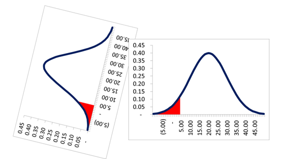
Q Mean 20 Mn$, volatility 10 Mn$. Normal VaR calculation at 5% significance
1) 5 % probability of losses of atleast 3.5 Mn$
2) 5% probability of earnings of atleast 3.5 Mn$
3) 95% probability of losses of atleast 3.5 Mn$
4) 95% probability of earnings of atleast 3.5 Mn$

My method
Var (5%) = -10 + 1.65*10 = -3.5 Mn $
Therefore loss is -3.5 Mn$ but since it is negative it is basically earnings of 3.5 Mn $
At 95% confidence this is the maximum earnings or at 5% this represents the minimum earning.

Therefore answer should be 2)5% probability of earnings of atleast 3.5 Mn$
However answer given is 4) 95% probability of earnings of atleast 3.5 Mn$

Am i missing a trick somewhere?

Many thanks in advance for the help
KR
Uzi

 

[David Harper CFA FRM]

Hi @monsieuruzairo3

I am not crazy about the question, but I like your VaR calculation, that's the way to do it. And the negative result (-3.5) is atypical: as you say, it implies a gain, not the typical loss. So it's only your interpretation that goes a little wrong, i think. Go back to when we typically calculate a VaR, call it "L". If the 95% VaR is L, we mean either: 95% of the time the loss will not exceed L, or 5% of the time we expect the loss to exceed L. This question is reverting from L/P to P/L where loss "is on the left" (where it's more natural anyway, this question seems to be confusing only insofar as it reverts to our more typical expectation of a -/+ axis). So, as I plotted below, this question implies a (simple) distribution with mean of +20 and sigma 10, such that 95% of outcomes would be greater than +3.5 or 5% would be less than +3.5. So (D) looks correct, although I don't think it's a fantastic question as-is. Thanks,

 

[monsieuruzairo3]

Hi @David Harper CFA FRM CIPM
Thanks for the response. I got your point!
One more thing related to market risk
Ch: The art of term structures models: drift
Doubt related to model 1,2
Model dr= sigma *dw
As per Schweser if dw= 0.2, sigma =1.2% then dr= 0.24%
Model 2 Bionic turtle r =4%, sigma=2.5%, dw=.80642, dt=1/12, drift 1%
dr= 4+(1/12)+2.5*.80642*sqrt(1/12)
My question is why have you multiplied dw by sqrt of dt??
I got really confused seeing BT question and Scheweser one. Am I misinterpreting something drastically?
Thanks in advance
Uzi

 

[David Harper CFA FRM]

Hi @monsieuruzairo3 it's hard when you don't tell me what question/note you are referring to but, as far as I can see, that refers to question T3.406 (?) @ https://forum.bionicturtle.com/thre...endent-interest-rate-volatility-model-3.6721/
(if i'm wrong, please let me know?) ... including ...

She makes the following assumptions:

• The time step is monthly, dt = 1/12
• The initial short-term rate, r(0) = 4.00%
• The annual basis point volatility = 3.00%
• The annual drift, lambda(t), is constant at 130 basis points (+1.30%) per year
• The alpha parameter = 0.380

Her simulation extends over a 10-year horizon. For the 60th month, the random uniform [0,1] value is 0.20 such that (via inverse transformation) the random standard normal = NORM.S.INV(0.20) = -0.8416; and dw = -0.8416*SQRT(1/12) = -0.2430 (note: the exam is unlikely to go into such detail on dw, we show this math simply to remind that dw is not a standard random normal, but rather an already-time scaled random normal)

In these term structure models, the general form indeed is given by dr = [...] + σdw, where σdw is the random shock. So, of course I agree with Model 1: dr= sigma *dw. In my calculations above, I have 0.80642 as a random standard normal, N(0,1), which is multiplied by SQRT(1/12) to produce dw, because dw is a random (non-standard) normal with mean of zero but standard deviation of sqrt(dt). In this way, your suggestion is correct: dw is already time-scaled, or put another way, incorporates the sqrt(dt).

It's maybe helpful to parse the dw explicitly:

dr = [...] +σ * dw
dr = [...] +σ * [ Z * sqrt(t)]

To see that, essentially, this shock component takes a random standard normal, Z = random N(0.1), and multiplies it by σ * sqrt(t) which is a per annum volatility ("annual basis point volatility" is the conventional input!) scaled by time. I hope that explains, thanks,