Hypothesis Test : Calculating P Value

atandon

Member
Hi David,

Could you pls clarify my doubt stated below -

When we did the hypothesis test in VAR chapter and calculated the t-statistic value, we always use to compare it with critical/look up value based on confidence level to make a call whether to reject or accept the hypothesis. So we were getting away in calculating the p-value here.

But when we reached linear regression chapter - we don't have a confidence level. So when we performed the hypothesis test and calculated our t-statistic number and let's presume it comes (as you said on the video) around 2 and 3 which is our sweet spot, we have to make a call to reject/accept from the p-value. My question is - how should we calculate the p value from t-statistic number and how to interpret the p-value once we have it?

Many Thanks,
atandon
 

Aleksander Hansen

Well-Known Member
From what I understand, you will not have to calculate the p-value (directly); simply know the critical values for key percentiles.
For a t I would think that you would be provided a table due to the degrees of freedom issue, OR that the values will be high or low enough for you to infer whether to accept or reject. The calculation is non-trivial unless you have certain t-values, or a lookup table.
I'm sure David will correct me if I'm incorrect.
 

David Harper CFA FRM

David Harper CFA FRM
Subscriber
I agree entirely with Aleks comment.

I think it helps to see the p-value (at least in tests of sample mean, which includes tests of regression coefficients as they are effectively sample means) as the distributional CDF; e.g., if the sample mean is +/-1.645 standard deviations from the hypothesized population mean, the one-tailed p-value is ~5% and the two-tailed p-value is ~10%. The computed t-statistic is the number of standard deviations separating an observed mean from the hypothesized mean, and the p-value is just the area in the reject tail(s). For this reason, the p-value is no different to calculate (not easier than) finding N(.) in BSM. It's just the area in the tail(s); once I really saw that, then I realized that the header row in the lookup tables are p-values (such that the lookup tables can be used in reverse to find p-values).

So, just as Alek says, its possible you are given a table ... My question #2 shows what a table snippet might look like: http://forum.bionicturtle.com/threads/mock-2012-p2-1-1-5-market-risk.5729/

I think you only need to know: 1.645 and 2.33 (one tailed 95% and 99%) and 1.96 and 2.58 (two tailed 95% and 99%). VaR is always the one-tailed; most significance tests (e.g., regression means) are often the two-tailed.

If you can comprehend the p-value visually, you will see why we can reject outright, for sheer example, a t-statistic of 13.7 if you have a large enough sample (a common mistake is to look this up or get stuck...). It means the sample mean is 13.7 standardized standard deviation from the (null) hypothesized mean: a very large distance --> a very small area in the tail(s) --> a very small p-value. It's an outright reject just from a mental image. I hope that helps,
 

Jaskarn

Active Member
Hi David,

Please help in understanding how we reached P values 30% for 1 Tail and 60% for 2 tail. step by step

p-values.JPG
 

David Harper CFA FRM

David Harper CFA FRM
Subscriber
Hi @Jaskarn If you understand the computed t value, there's only one step. The computed t-value (aka, test statistic) of 0.54 is given (as already shown) by (45 - 40)/9.262 where 9.262 is the standard error and its calculation is also shown as 29.28/sqrt(10) = 9.262. I think many people skip over the interpretation of this test statistic of the sample mean (i.e., the 0.54) but it's super helpful to understand what it means. Otherwise we are at the mercy of too many numbers.

The observed sample mean is 45.0 and our null hypothesis is 40.00. This means our observation is a raw distance of (45.0 - 40.0) += 5.0 way from where we hypothesize the true (population) mean to be. That's (X - μ) = 5.0. How far is that? We can't say until we standardize this raw distance. To standardize is to compute (X - μ)/σ = (45 - 40)/9.260 = +0.54; the raw distance of +5.0 is +0.54 standard deviations away from our (null) hypothesized mean. (We might even say it is +0.54 standardized standard deviations because we can compare this to other test statistics via the lookup table). Although we use the student's t here, technically, we can approximate with the normal because its a large (n>30) sample and this is the intuition: our observation of 45.0 is only +0.54 standard deviations above the "suspected" (null) hypothesis and, right away, we know this is not far enough to land in the rejection region. This is too near to the null: random sampling variation (aka, luck) could easily produce such a small difference. We know we will not be rejecting.

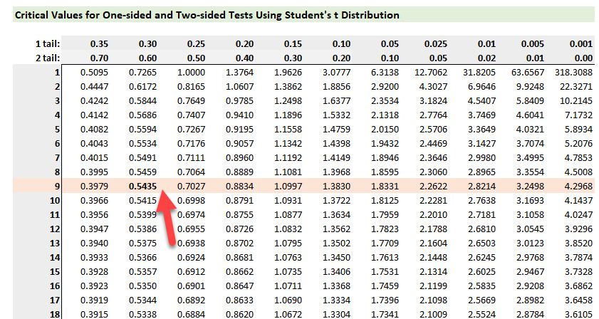
Below is a student's t lookup, except I added columns to the left. The answer to your question is that there is only one step. Given a 9 df and a t-statistic of 0.54, in Excel, the 2-sided p-value = T.DIST.2T(0.54, 9) = 0.6023 and the 1-sided p-value = T.DIST.RT(0.54, 9) = 0.31165. On the student's t distribution with 9 df, at the +0.54 quantile, the area to the right (under the pdf curve) is fully 30% of the curve (!) such that, if we count both tails, 60.2% of the area is in the rejection regions; i.e., under 1-sided ~ 69.9% of the area is "to the left" in the acceptance region and under 2-sided only ~39.8% is "inside" in the acceptance region. This is reflected in the lookup table below, except we invert and find the 0.54 in the interior, which is nearest o the 0.5435. Looking up to the top header row, we see that 0.5435 corresponds to 0.30 1-tailed and 0.60 2-tailed; this are corresponding p-values. I hope that's helpful,

082120-students-t2.png
 
Top