Gujarati-Skewness/Kurtois Calc formula & clalrification

[PDEM200]

Hi David,
Could you please provide some guidance on the following:

1) Sample Skewness and Kurtosis Formulas

I have seen 2 differnt versions,can you please clarify which is correct:

Version#1: Sample Skewness

Sum of Third moment about the mean / cube of Std Deviation * 1/ N

Version#2:
[ [ Sum of Third moment about the mean] / (n-1) ] / cube of Std Deviation

Which one is correct?

2) In Gujarati 3.8, can you please provide additional details concerning the use/purpose of the Alternative Skew and Kurtosis calculation that is provided.

Thank you

 

[David Harper CFA FRM]

Hi Paul,

If by "Sum of Third moment about the mean" you mean "Sum of [X - mean]^3" then your #1 appears to me to be the population skew:
[Sum of [X-mean]^3 / n ] * 1/StdDev^3 = E[(x-mean)^3] / StdDev^3 = Population third moment / StdDev^3
i.e, that looks to match the skew when n = entire population size
or, note Gujarati's 3.10: the six-sided die is fully characterized by the uniform PDF. That's not a sample, it's an expectation, so there is he is right to use population (sum and divided 6). Put another way, your #1 is fine for a population (unrealistic if historical) or if, ex ante, we have a distribution that fully characterizes *expectation* the random variable (e.g., our expectations for a 6 sided die are not a sample)

While #2 is Gujarati's sample skew:
Sample third moment / StdDev^3
i.e., this for when we only have a sample (any realistic exercise where we use historical data is effectively a sample)
this is analogous to using Sum of [x - mean]^2 / (n - 1) for sample variance instead of divide by (n) for population.
the net effect is a slightly larger sample skew.

but caution: it's not "wrong" to use #1 on a sample, like it's not wrong to use (n) in denominator. These are estimators. There can be more than one. Using #1 is "incorrect" to Gujrati's sample but it is still an *estimator* of skew...

Here is the learning XLS on skew/kurt: http://www.bionicturtle.com/premium/spreadsheet/2.a.2._skew_kurtosis/

please note i have 2 sample skew/kurt cacs:
1. Gujarati's which matches your #2
2. The excel sample skew which is different than either (yes, it's a 3rd variation!) which adjusts for small sample bias. Just another estimator (this one "unbiased"). Note how similar they are...

for the actual data on Google returns, i get .107 sample skew (your #2, our "proper" sample skew) versus .108 "unbiased" sample skew (not your #1, which would be smaller, this is larger). The 1/100th difference is precision not justified by the reality of the distribution, we are lucky if we are in the rough neighborhood.

Hope this helps, David

 

[Eustice_Langham]

Hi David, I was about to start a new thread on this matter but saw this question/answer, so if I may clarify something with you.

For a sample when calculating skewness will the denominator always be calculated as std dev ^ 3 OR for a sample will the skewness denominator be std deviation ^ (3/n-1)

 

[Eustice_Langham]

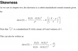
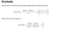
Hi David, I have a question re Skewness and Kurtosis that I have asked elsewhere. I have attached two screenshots of the calculations, I was of the understanding that given that Skewness and Kurtosis are the third and fourth moments respectively that the numerator and denominator are raised to the third and fourth powers respectively. That said I have seen some instances whereby the denominator is calculated differently. Looking at the denominator calculations, for Skewness the denominator calculation is raised to (3/2) and for Kurtosis the denominator calculation is raised to (2/2). Can you explain why this is the case and when should these calculations be used? Thankyou

 

[David Harper CFA FRM]

Hi @Eustice_Langham Like variance has a population estimate (aka, parameter) versus a sample estimate (aka, statistic), so do skew and kurtosis. Your displays are correct for skew, but they signify population skews. GARP's 5.9 and 5.10, although they are discussed in sample moments chapter, are really population moments. That's because they employ E(X) rather than X̅. E(X) implies we know the population's distribution. Here is a super simple example, a Bernoulli: Pr(X = 0) = 0.30 and P(X = 1) = 0.70. What is the skew of this Bernoulli?

The third central moment (aka, 3rd moment around the mean) is given by E[(X - μ)^3] = 30%*(0 - 0.70)^3 + 70%*(1 - 0.70)^3 = -0.0840; notice I used Greek μ because we have a population mean rather than a sample mean. We standardize it by dividing by σ^3; in this case then, skew = -0.0840 / σ^3 = -0.0840 / σ^3. What is σ^3? The (population) variance here is E[(X - μ)^2] = 30%*(0 - 0.70)^2 + 70%*(1 - 0.70)^2 = 0.210 such that the standard deviation = σ = sqrt(0.210) = 0.458258. The denominator (to standardize the third central moment) is σ^3, so here it σ^3 = 0.458258^3 = 0.09623409 and so the skew = -0.0840 / σ^3 = -0.0840 / 0.458258^3 = -0.8729.

But in this case it's easier to use the fact that σ^3 = (σ^2)^(3/2) per exponential property (x^n)^m = x^(n*m). Applied, skew = -0.0840 / (σ^2)^(3/2) = -0.0840 / 0.210^(3/2) = -0.8729. We never needed to compute a sample estimate here: we have fully informed expectations, E(.), because we know the population's distribution. Please do check my math, I'm writing quickly ...

On the other hand, if we just observed a sample = {0, 1} or for that matter here is a sample, {0, 0, 0, 1, 1, 1, 1, 1, 1, 1}, where the mean is also 0.30, X̅ = 0.30, but it's a sample mean and our sample skew will be larger (in absolute value) because the sample skew has an adjustment, similar to how sample variance divides by (n-1) instead of (n). I have a video on skew vs sample skew here at https://forum.bionicturtle.com/threads/t2-6-the-skew-and-sample-skew-of-a-distribution.21737/ which reconciles Excel's population skew, SKEW.P(), with its sample skew, SKEW(). I hope that's helpful,

 

[Eustice_Langham]

Thanks David