Forward Rate Formula

[FutureFRM]

I came across two different forward rate formula (Equation1 and 2 shown in attached screenshot). would like to know which formula is more “realistic“ and which to use in the exam. would appreciate if anyone can explain the differences too.

 

[David Harper CFA FRM]

Hi @FutureFRM We have already much discussion on this topic of implied forward rates (e.g, this may be helpful https://forum.bionicturtle.com/threads/shortcut-to-forward-rates-if-you-have-bond-prices.4927). There is only one concept here (ie, the rollover comparison at the top of your post, 37.5) but the difference is simply the compound frequency assumption. Your first formula derives from continuous compound frequency, while your second derives from semi-annual compound frequency. For this reason, strictly speaking, the first example should specify the continuous assumption: otherwise several answers are possible. Specifically, consider:

1. Assume z(1.0) = 2.1360% and z(2.0) = 2.9150% with continuous compounding, then f(1.0, 2.0) = (2.1950%*2 - 2.1360%)/1 = 3.6940%
2. Assume z(1.0) = 2.1360% and z(2.0) = 2.9150% with semi-annual compounding; this could be written "s.a. Z(1.0) = 2.1360%" or "Z(1.0) = s.a. 2.1360%", then s.a. f(1.0, 2.0) = [(1+2.9150%/2)^4/(1+2.1360%/2)^2 - 1]*2 = 3.6970%
3. Assume z(1.0) = 2.1360% and z(2.0) = 2.9150% with annual compounding, then: f(1.0, 2.0) = (1+2.9150%)^2/(1+2.1360%) - 1 = 3.69994%.

I don't know about realistic (exam questions should always be precise) except that certain financial instrument imply their own compound frequency; e.g., a 90-day Eurodollar futures settlement price of 99.50 implies LIBOR of 0.50% with quarterly compounding. Thanks,

 

[Matthew Graves]

Rather than trying to memorise these specific formulae, I find it much easier to remember the basic, underlying concept is the same for both in discount factor/growth factor space:

\[ GF(0,T_2)=GF(0,T_1)*GF(T_1,T_2) \]

Then, depending on the question or data provided you just need to calculate the various discount factors appropriately. As David says above, the only difference between the two approaches is the compounding frequency and therefore discount (or growth) factor calculation.

As an aside, I should say that I find the presentation of the continuously compounded case in the screenshot confusing. Maybe I am just missing the associated background text to the numbers but my assumption would be that the quoted values would be the annual, continuously compounded rate. I therefore find the dividing by 2 and then multiply by 4 misleading. The general form is:

\[ GF=e^{rt} \]

where r is the annual continuously compounded rate and t is the period length in years. The full equation should therefore be:

\[ e^{0.02915*2}=e^{0.02136*1}*e^{r*1} \]

Obviously this works out the same but I don't see the rationale for the way it is presented in the text.

 

[David Harper CFA FRM]

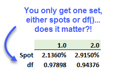
Hi @Matthew Graves great points and advice, thank you! Like you, I find the exponentiation of x/2*4 above confusing. I used this example in a recent LinkedIn post (here https://www.linkedin.com/posts/bionicturtle_frm-riskmanagement-frm-activity-6595354453270949888-jgzr) to illustrate the ambiguity of a spot rate that is given without its corresponding compound frequency; e.g., "the two-year [spot] rate is 2.915%" is ambiguous, we need to be told "the two-year [spot] rate is 2.915% with semi-annual compounding." However, discount factors never lie:

Unlike ambiguous 2.9150%, the df(0.94376) conveys only a single rate. And I like the elegance of how we can retrieve the forward rate with f = ln[df(1.0)] - ln[df(2.0)] = ln(0.978980) - ln(0.943760) = 3.6639% per:

• Since df(1.0) = exp(-z1*1) and df(2.0) = exp(-z2*2),
• ln[df(1.0)] = -z1 and ln[df(2.0)] = -z2*2; or
• z1 = -ln[df(1.0)] = and z2 = -ln[df(2.0)]/2; e.g.,
  • z1 = -ln(0.97890) = 2.12441%, and
  • z2 = -ln(0.943760)/2 = 2.89417%
• Because exp(z1*1)*exp(f*1) = exp(z2*2) -->
• forward, f = z2*2 - z1, so that:
• f = ln[df(1.0)] - ln[df(2.0)] = ln(0.978980) - ln(0.943760) = 3.6639%

These rates--i.e., z1 spot of 2.12441%, z2 spot of 2.89417%, and one-year forward of 3.6639%--are with continuous compounding and of course they can be translated into their equivalent annual/semi-annual discrete rates, but unlike the "2.1360%", they would be translations of a single rate! Thanks,

 

[FutureFRM]

Thank you @David Harper CFA FRM @Matthew Graves ! These are all very helpful in enhancing my understanding on forward rate. However, I still have one questions regarding the appropriate rate to calculate the cash flow in interest rates swap using FRA method.

In the example below, the forward rate needs to be computed from the spot LIBOR rate at 9 and 15 months in order to calculate the cash flow of floating leg.




However , In Q34, no forward rate is needed here. Is that because we are at Aug 9, 2014, which means we can simply take the 6-month LIBOR rate as of Feb 9,2016?

 

[David Harper CFA FRM]

Hi @FutureFRM The difference is that GARP 2018 P1.34 question is not showing a table of current (as of Aug 9, 2014) spot rates; it's easy to get this wrong because we are accustomed to seeing a table (term structure) of spot rates, but the exhibit in 34 is not a term structure of spot rates! Instead, the table illustrates the future of actual, realized six-month LIBOR rates because the question is largely testing us to know that in a vanilla IRS the rate is observed at the beginning of the period but paid at the end of the period. The table is a "simulation" of six-month rates, instead of a term structure (of 0.5, 1.0, 1.5, 2.0 etc) spot rates. Thanks,