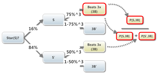
Here is a recent question I wrote to test Bayes Theorem (which has been reintroduced into the FRM)
1. Tree Approach
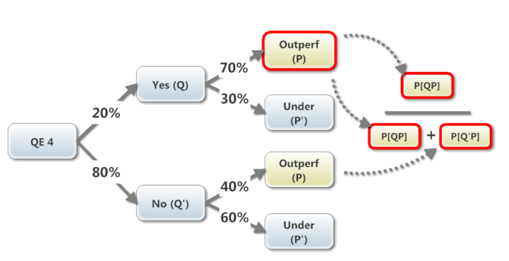
I have typically used a (binomial) tree to visualize this sort of problem. You start the tree with the unconditional (aka, marginal) probabilities which are the probabilities that do not depend on anything else; in this case, the unconditional probability of a QE 4 is 20%, the conditional probability of fund outperformance, Prob[P|Q] = 70%, and their joint Prob[QP] = 20%*70%=14%:
The Bayes (posterior but still conditional) probability question asked is, what is the probability of QE 4 (Q) given that we observe Outperformance (P), Prob(Q|P). It's just the "reverse" of the conditional probability that happens to be supplied by the question: we are given that Prob(P|Q) = 70%, but we want Prob(Q|P).
The tree let's us visualize how Bayes works: Prob(Q|P) is the probability of the joint outcome, Prob(QP), in the numerator, divided by all of the events that include outperformance, Prob(P), which here only includes two: Prob(QP) + Prob(Q'P). Visually, the two yellow nodes constitute all possible nodes that include outperformance (P), so that is our denominator. Now, if we observed (Q) has happened, then the conditional probability that (P) also happens is the same as the joint Prob(QP), so that is the numerator.
2. Probability Matrix
Miller (new to the FRM) employs these handy probability matrixes which, it seems to me, give us another way to grasp Bayes (it's not mechanically any different, I'm sure it's been done somewhere, i just haven't seen it ....).
In the probability matrix approach, here are the question's same setup assumption rendered into cells:

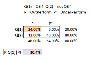
All we need to do is produce the "probability matrix" which in Miller simply means a matrix of joint probabilities. In a joint probability matrix, all of the body cells sum to 1.0. For example, Joint Prob[Q(1),P]=20%*70%=14%; Joint Prob[Q(1),P']=20%*30%=6%; Joint Prob[Q(2),P]=80%*40%=32%. Here is the implied joint probability matrix:
Once the problem's assumptions are "translated " into a joint probability matrix, I find the Bayes Theorem question relatively easier to grasp: the Prob[Q | P] is simply the conditional probability retrieved from the matrix.
Our information is that (P) occurred: this implies our outcome must be located in column (P) which has an overall probability of 46.0% (Our prior information is that P happened and P' did not) . As our joint outcome is the upper cell Prob[Q(1),P] = 14%, our desired Bayes' conditional probability, Prob [Q(1)|P], is simply divides the joint probability cell by the column probability, Prob [Q(1)|P] = 14%/46% = 30.4%.
Question: 302.1. There is a prior (unconditional) probability of 20.0% that the Fed will initiate Quantitative Easing 4 (QE 4). If the Fed announces QE 4, then Macro Hedge Fund will outperform the market with a 70% probability. If the Fed does not announce QE 4, there is only a 40% probability that Macro will outperform (and a 60% that Acme will under-perform; like the Fed's announcement, there are only two outcomes). If we observe that Macro outperforms the market, which is nearest to the posterior probability that the Fed announced QE 4?
1. Tree Approach
I have typically used a (binomial) tree to visualize this sort of problem. You start the tree with the unconditional (aka, marginal) probabilities which are the probabilities that do not depend on anything else; in this case, the unconditional probability of a QE 4 is 20%, the conditional probability of fund outperformance, Prob[P|Q] = 70%, and their joint Prob[QP] = 20%*70%=14%:

The Bayes (posterior but still conditional) probability question asked is, what is the probability of QE 4 (Q) given that we observe Outperformance (P), Prob(Q|P). It's just the "reverse" of the conditional probability that happens to be supplied by the question: we are given that Prob(P|Q) = 70%, but we want Prob(Q|P).
The tree let's us visualize how Bayes works: Prob(Q|P) is the probability of the joint outcome, Prob(QP), in the numerator, divided by all of the events that include outperformance, Prob(P), which here only includes two: Prob(QP) + Prob(Q'P). Visually, the two yellow nodes constitute all possible nodes that include outperformance (P), so that is our denominator. Now, if we observed (Q) has happened, then the conditional probability that (P) also happens is the same as the joint Prob(QP), so that is the numerator.
2. Probability Matrix
Miller (new to the FRM) employs these handy probability matrixes which, it seems to me, give us another way to grasp Bayes (it's not mechanically any different, I'm sure it's been done somewhere, i just haven't seen it ....).
In the probability matrix approach, here are the question's same setup assumption rendered into cells:

All we need to do is produce the "probability matrix" which in Miller simply means a matrix of joint probabilities. In a joint probability matrix, all of the body cells sum to 1.0. For example, Joint Prob[Q(1),P]=20%*70%=14%; Joint Prob[Q(1),P']=20%*30%=6%; Joint Prob[Q(2),P]=80%*40%=32%. Here is the implied joint probability matrix:

Once the problem's assumptions are "translated " into a joint probability matrix, I find the Bayes Theorem question relatively easier to grasp: the Prob[Q | P] is simply the conditional probability retrieved from the matrix.
Our information is that (P) occurred: this implies our outcome must be located in column (P) which has an overall probability of 46.0% (Our prior information is that P happened and P' did not) . As our joint outcome is the upper cell Prob[Q(1),P] = 14%, our desired Bayes' conditional probability, Prob [Q(1)|P], is simply divides the joint probability cell by the column probability, Prob [Q(1)|P] = 14%/46% = 30.4%.

