What’s Wrong with Multiplying by the Square Root of Time?

[emilioalzamora1]

Hi All,

I just wanted to share an important topic which is unfortunately completely neglected in the GARP curriculum.

Under the assumptions of i.i.d we know that the following properties apply to the scaling of mean and variance (volatility) - I am referring to C. Alexander 'Market Risk Analysis' here:

Given a certain annualizing factor 'A' (let's say A equals 12) we want to convert monthly returns (A = 1) into annual returns (hence, the annualising factor of 12, A = 12):

1. μA >> mean scales proportionately with the annualizing factor A (Mu times A)

2. σ^2A >> variance scales proportionately with the annualizing factor A (sigma squared times A)

3. σ*sqrt(A) >> standard deviation scales disproportionately with the the square root of the annualizing factor A (sigma times the square root of A)

Morningstar has published the following note about 'What’s Wrong with Multiplying by the Square Root of Twelve' talking about the original formula proposed by Tobin (1965) and how to more appropriately scale variance (volatility):

For all of those interested: I did some random manipulation and in line with the theory it reveals that scaling with the 'square root rule' will underestimate standard deviation.

The formula for the variance goes like this. Assume we have calculated the variance over a given time period simply given below as σ^2 (at t:0) on the right-hand side while
on the left-hand side we have σ^2 (the scaled variance at t:1) to be clear about the notation:

σ^2(scaled for 'n' periods) = [ { σ^2 + (1+μ)^2 }^n - (1+μ)^(2*n) ]

If we wish to scale monthly variance to annual variance, 'n' in the above formula is 12 and in the right-hand side of the equation 1+mu is raised to the power of (2*12).
Notice, we can also use 'A', the annualising factor, in the formula above to be in line with C. Alexander.

Hope this is helpful.

I have attached the paper here: https://corporate.morningstar.com/U...ents/MethodologyPapers/SquareRootofTwelve.pdf

 

[David Harper CFA FRM]

Hi @emilioalzamora1 Awesome share on an important topic, thank you! I just read the paper, it does indeed illustrate the interesting implications of scaling simple (aka, arithmetic) returns rather than log (aka, geometric) returns. Please note it does admit that the square root rule is valid for i.i.d. log returns, as in LN(S2/S1). By convention, simple returns, as in S2/S1-1, are often treated as approximations of log return (e.g, Hull does exactly this and says so in his volatility calculation). Hence the bias.

I am glad you mentioned Carol Alexander because our first learning XLS (R1-P1-T1-Intro-VaR.xlsx) implements her adjusted volatility/VaR where the adjustment is a scaling factor that alters the square root rule. This refers to what I would consider the more important issue concerning (ie, What's Wrong with ...) the Square Root Rule, which has been discussed in this forum for years: its key assumption is i.i.d. returns. The "independence" in i.i.d. implies zero autocorrelation ("identical" implies constant variance).

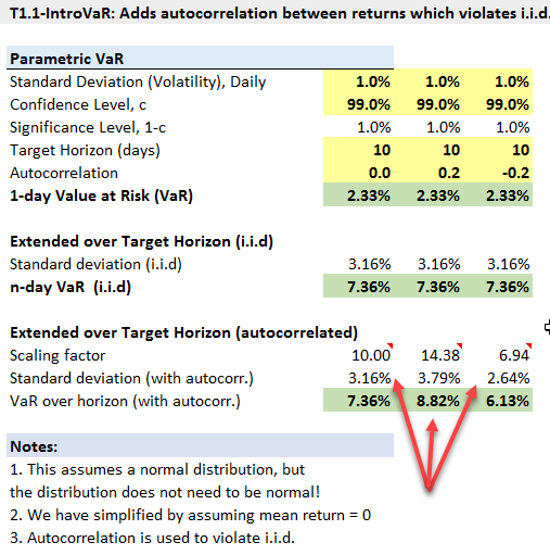
Below I copied the relevant section from C. Alexander (emphasis mine) plus a screenshot from my learning XLS which implements her scaling adjustment. It is a popular but mistaken view that the key SRR assumption is normality, but the distributional assumption is far looser, the critical assumption is i.i.d. and that's why good questions should state this assumption. The reality is that we are routinely assuming i.i.d. for the sake of convenience.

Please notice in my screenshot illustration there are three columns, the inputs are identical except for the autocorrelation assumptions:

• In the first column, our typical approach: daily 1.0% volatility is scaled over 10 days such that 10-day vol = 1.0%*sqrt(10/1) = 3.16%
• In the second column, autocorrelation = +0.2 such that the 10-day vol = 3.79%
• In the third column, autocorrelation = -0.2 (aka, mean reversion) such that 10-day vol = 2.64%. You can see, scaling per SRR can either over- or under-state

And this is consistent with Linda Allen, which has been in the P1.T4 syllabus actually for over ten years (yikes!). So the FRM syllabus has been aware of this for long time, actually. Specifically,

Mean reversion has an important effect on long-term volatility. To understand the effect, note that the autocorrelation of interest rate changes is no longer zero. If increases and decreases in interest rates (or spreads) are expected to be reversed, then the serial covariance is negative. This means that the long horizon volatility is overstated using the zero-autocovariance assumption. In the presence of mean reversion [david harper: mean reversion = negative autocorrelation] in the underlying asset’s long horizon, volatility is lower than the square root times the short horizon volatility." -- Linda Allen Chapter 2

Here is C. Alexander:

"II.3.2.2 Constant Volatility Assumption
The assumption that one-period returns are i.i.d. implies that volatility is constant. This follows on noting that if the annualizing factor for one-period log returns is A then the annualizing factor for h-period log returns is A/h. Let the standard deviation of one-period log returns be σ. Then the volatility of one-period log returns is σ*sqrt(A) and, since the i.i.d. assumption implies that the standard deviation of h-period log returns is σ*sqrt(h), the volatility of h-period log returns is σ*sqrt(h) * sqrt(A/h) = σ*sqrt(A).

In other words, the i.i.d. returns assumption not only implies the square-root-of-time rule, but also implies that volatility is constant. A constant volatility process is a fundamental assumption for Black–Scholes–Merton type option pricing models, since these are based on geometric Brownian motion price dynamics. In discrete time the constant volatility assumption is a feature of the moving average statistical volatility and correlation models discussed later in this chapter.

But it is not realistic to assume that returns are generated by an i.i.d. process. Many models do not make this assumption, including stochastic volatility option pricing models and GARCH statistical models of volatility. Nevertheless the annualization of standard deviation described above has become the market convention for quoting volatility. It is applied to every estimate or forecast of standard deviation, whether or not it is based on an i.i.d. assumption for returns." -- Carol Alexander, page 92, Vol II MRA

 

[emilioalzamora1]

Excellent reply! I will add another couple of points over the next few days.

 

[emilioalzamora1]

Hi David,

as promised I want to clarify a few things here.

First of all you don't mention that the Annualization Factor is calculated using the attached (copied) formula; to be precise the so called Annualization Factor involves the square root. Hence as in your post would be 3.16%, 3.79% and 2.64% respectively.

The next point we need to be clear about is for what 'h' in the formula stands for:

Comparing the following two examples used in C. Alexander: 1.) Annualization Factor for estimating Vol. for hedge Funds (book Market Risk, example II.3.2) 2.) Volatility-Adjusted Sharpe Ratio (which uses the exactly same Annualization Factor in her book Quant. Method, example I.6.12)

ad 1.) assumes monthly returns which are then 'scaled' to annual returns, hence h = 12
ad 2.) assumes daily returns which are then 'scaled' to annual returns, hence h = 252 (or 250 if you wish)

[In the above example, compiled by David, we have daily standard deviation (or 1-day VaR) 'scaled' for 10 days, hence h = 10]

I would like to further extend this discussion to the Lo (2002) paper 'The Statistics of Sharpe Ratios' (paper copied below): Figure1 (on page 41) shows the effect of pos/neg/zero autocorrelation on Sharpe Ratios.
I am not 100% sure about equation (22). This is apparently a different Scale Factor (Annualization Factor) than the one used by C. Alexander.
Would be great to have some discussion about it.

Many thanks!

http://edge-fund.com/Lo02.pdf

 

[David Harper CFA FRM]

Hi @emilioalzamora1 Thank you! Yes, you are correct: the scaling factor in my XLS is the same as Carol Alexander's simply because that is where I got it (it has never appeared in an assigned FRM syllabus, eg)! The Lo paper looks interesting, his #20 to #22 appear to bear similarities ...