Blog Week in Risk (ending Dec 11th)

[David Harper CFA FRM]

New content added to the Study Planner this week (selected only)

Thanks to great help from @Nicole Seaman and Deepa, we are in a terrific position with respect to updating our program for the 2017 FRM syllabus. Our initial emphasis is the study notes and underlying (learning) spreadsheets. You may not be aware but I keep updated spreadsheets for almost every quantitative concept in the FRM; this allows me to be maintain rigor and fact-check practice questions. We plan to update the entire library of videos for the 2017 syllabus, also. Finally, the fresh practice question discipline will resume right after the new year. In the last week we published significant revisions to the following Study Notes

• Diebold’s Elements of Forecasting (R15.P1.T2 Chapters 5, 6, 7 and 8). This is one of the FRM’s hardest readings. The problem--and the syllabus weakness (in my opinion, of course)--is the isolated, theoretical presentation of this time-series material. It is almost impossible to master this material without engaging in actual data and applications. As evidence, I'd point to the EOC Q&A which is basically applications. MS Excel is necessary but increasingly not sufficient. I have thoughts about how to do this. In the background I have started to gradually build R-based (best hashtag is #rstats) examples to complement our spreadsheets. Diebold uses eViews, which is a great tool. But years ago I began my own investment in learning R (https://www.r-project.org/) as my data science language of choice. And currently, it does seems like R and Python are the leading data science languages. Obviously everybody cannot become a coder or data scientist, which requires a significant and sustained commitment level. However, I do think every manager will need to become at least data-savvy and further, risk managers should aspire to be at least novice (part-time?) data scientists.
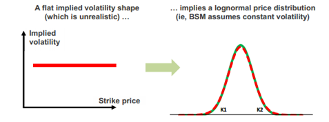
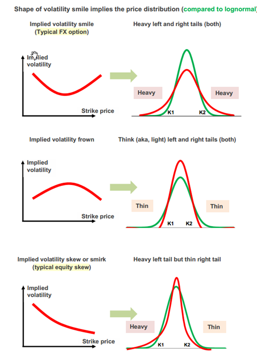
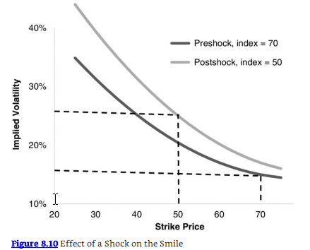
• Hull’s Chapters (R40.P2.T5) on the Risk-free rate (OIS) and Implied Volatility. Additional comments below (here).
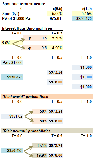
• I spent the last four or five days meticulously updating (R39.P2.T5) Tuckman’s Term Structure chapters. Additional comments below (here).

Banks

• China’s Banks Are Hiding More Than $2 Trillion in Loans http://www.wsj.com/articles/chinas-banks-are-hiding-more-than-2-trillion-in-loans-1481130392 "The surge shows how Chinese banks are trying to keep the credit spigot open to support the country’s slowing economy. Structuring financing deals as investments instead of loans frees up bank capital and makes it easier to extend loan deadlines or new credit to borrowers … If Chinese banks were required to count their investment receivables as loans, the banks would need to raise as much as $212 billion in capital, estimates UBS analyst Jason Bedford. That is not far short of the $262 billion raised by all Chinese banks in 2015.”

Political and regulatory (including BIS)

• BIS Quarterly Review, December 2016 https://www.bis.org/publ/qtrpdf/r_qt1612.htm
• Assessing consistency of implementation of Basel standards http://www.bis.org/bcbs/implementation/l2.htm “With today's publication of reports that assess the implementation of Basel standards in Indonesia, Japan and Singapore, the Basel Committee on Banking Supervision has completed its review of the implementation of the risk-based capital framework by all of its members.”
• Summing It Up: A Brief History of the Economy, Regulations, and Bank Data (by Federal Reserve Bank of Atlanta) https://frbatlanta.org/economy-matt...ewpoint/2016/12/06/history-of-bank-regulation

Technology (including FinTech and cybersecurity)

• U.S. Commission Finds Lack of ERM Is Cybersecurity Weakness http://www.garp.org/#!/risk-intelligence/technology/cyber-security/a1Z40000003NFb4EAG Report is here http://trtl.bz/2hpHOhO

Exams (GARP, FRM, CFA) and Careers

• It’s Just No Fun Being a Swiss Banker Anymore (Heightened regulations, ultralow interest rates and a tech industry competing for talent have upended the profession) http://www.wsj.com/articles/the-swiss-banker-undergoes-a-tectonic-shift-1481106604

Climate (Matthew)

• Lloyd’s Finds Extreme Weather Can Be Accurately Modeled Independently http://www.riskmanagementmonitor.co...ther-can-be-accurately-modeled-independently/
• ClimateWise launches two reports that warn of growing protection gap due to rising impact of climate risks http://www.cisl.cam.ac.uk/business-...rn-protection-gap-due-to-impact-climate-risks

Books and Courses (including Journal/SSRN)

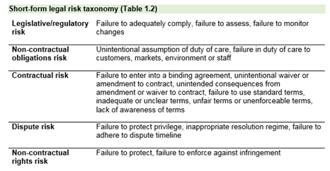
• [New Book] The Legal Risk Management Handbook: An International Guide to Protect Your Business from Legal Loss http://amzn.to/2gpS7Ai Contains this legal taxonomy:
  
  

Other

• Glass Lewis 2017 Proxy Season Guidelines http://www.glasslewis.com/2017-proxy-season-asian-guidelines-available/ Report is here http://trtl.bz/glass-lewis-us-guidelines-2017

Risk Foundations (FRM P1.T1) including enterprise risk management (ERM)

• Oliver Wyman Risk Journal Volume 6 http://www.oliverwyman.com/our-expertise/insights/2016/dec/oliver-wyman-risk-journal.html “Oliver Wyman today identified the top three risks facing global businesses in 2017 as it launches its 6th annual Risk Journal. The risks are: The re-emergence of nationalism and current political landscape; Technological change; and Cyberattacks” Report is here http://trtl.bz/oliver-wyman-risk-journal-no6
• Nomura Has 10 'Gray Swan' Risks That Could Roil Markets in 2017 https://www.bloomberg.com/news/arti...ey-swan-risks-that-could-roil-markets-in-2017 “7. A clearing house crisis: The systemic risks that stem from the clearing houses that were themselves introduced to contain systemic risks aren't new to regulators: financial stability watchdogs are already taking measures to deal with any potential fallouts. The interplay between struggling banks, collateral squeezes, sharp market moves in an overpriced market with central counterparties at the center could potentially lead to a crisis, in Nomura's worst-case scenario.”
• Cambridge Global Risk Outlook 2017 “CCRS identifies three important emerging trends in the global risk landscape: Emerging economies will shoulder an increasing proportion of risk-related economic loss as a result of both their accelerating economic growth and their increasing risk environment. Therefore, their risk environment is less stable; There is a growing prominence of manmade risks; A heavy contribution is expected from new or emerging risks, such as cyber attacks and infrastructure vulnerabilities.” Report is here http://trtl.bz/cambridge-global-risk-2017
• Lloyd’s City Risk Index 2015-2025 http://www.lloyds.com/cityriskindex/
• Enterprise Risk Management: Selected Agencies' Experiences Illustrate Good Practices in Managing Risk http://www.gao.gov/products/GAO-17-63 Report is here http://trtl.bz/gao-erm-dec16

Quantitative Analysis (FRM P1.T2)

• Introduction to K-means Clustering https://www.datascience.com/blog/in...tering-algorithm-learn-data-science-tutorials “K-means clustering is a type of unsupervised learning, which is used when you have unlabeled data (i.e., data without defined categories or groups). The goal of this algorithm is to find groups in the data, with the number of groups represented by the variable K. The algorithm works iteratively to assign each data point to one of K groups based on the features that are provided. Data points are clustered based on feature similarity.”

Financial Markets and Products (FRM P1.T3) including interest rates

• Time is Right for LIBOR Alternative https://www.financialresearch.gov/from-the-director/2016/12/08/time-is-right-for-libor-alternative/ “The ARRC [Alternative Reference Rates Committee] has narrowed the list of potential alternatives to two: A secured repurchase agreement (repo) rate and an unsecured rate, the Overnight Bank Funding Rate. A repo is essentially a collateralized, or secured, loan when one party sells a security to another party with an agreement to repurchase it later at an agreed price. Published by the Federal Reserve Bank of New York, the Overnight Bank Funding Rate is a broad, widely accepted measure of the cost of funds for U.S. banks based on the federal funds rate and those on overnight Eurodollar deposits.”
• The Man Who Invented the World’s Most Important Number (LIBOR) https://www.bloomberg.com/news/features/2016-11-29/the-man-who-invented-libor-iw3fpmed
• What’s up with the term premium? https://ftalphaville.ft.com/2016/12/01/2180569/whats-up-with-the-term-premium/
• Why Are Long-Term Interest Rates So Low? http://www.frbsf.org/economic-resea...mber/why-are-long-term-interest-rates-so-low/ “To understand why rates are low, it is useful to consider the two key components of long-term interest rates. The first is the average of expected future short-term interest rates—the expectations component. The second component is the term premium, which includes compensation to investors for the risk of holding long-term bonds but is also a catch-all for other factors beyond the expectations component that affect long-term rates.”

Valuation and Risk Models (Including Country Risk) (FRM P1.T4)

• About the challenges of sovereign risk modelling https://www.linkedin.com/pulse/challenges-sovereign-risk-modelling-bernhard-obenhuber
• Types of Financial Models (Top 4 in Investment Banking) http://www.wallstreetmojo.com/types-of-financial-models

Operational risk (FRM P1.T7)

• Top Security Threats to Companies in 2017 https://www.pinkerton.com/blog/top-company-security-threats-2017/ “Top Security Threat #1: Lone Wolf Attacks and Corporate Travel … Top Security Threat #2: Natural Disasters Packing More Punch”

Investment risk (FRM P1.T7) including pension crisis

• Is Private Company Ownership a Risk for Mutual Funds? http://news.morningstar.com/articlenet/article.aspx?id=783216 “This example highlights a risk of private-company ownership in an open-end structure. Investors can be fickle and may not stick around when the fund is going through a rough spell. Managers can be forced to trim or sell publicly traded stocks they may have preferred to keep. Portfolio construction can also appear out of whack, as the private, illiquid holdings soak up more of a fund's assets and drive more of the fund's performance than perhaps was initially intended.”
• A Dallas public pension fund suffers a run http://www.economist.com/news/finan...en-brewing-decades-and-it-not-confined-dallas “BANK runs, with depositors queuing round the block to get their cash, are a familiar occurrence in history. A run on a pension fund is virtually unprecedented. But that is what is happening in Dallas, where policemen and firefighters are pulling money out of their city’s chronically underfunded plan, and Mike Rawlings, the mayor, is suing to stop them … The crisis is the result of three linked issues: overgenerous pension promises; the flawed nature of public-sector pension accounting in America; and some bad investment decisions. In order to pay the generous benefits, the scheme counted on an investment return of 8.5% a year, absurdly high in a world where the yield on ten-year Treasury bonds has been hovering in a range of 1.5-3%. So the scheme opted for riskier assets in private equity and property. But the strategy did not work; the value of its investments declined by $263m in 2014 and $396m in 2015, thanks largely to write-downs of those risky assets.”
• South Carolina's looming pension crisis http://trtl.bz/2gB5Bwh

 

[David Harper CFA FRM]

Additional comment on updated Hull Chapter 20 (Volatility Smiles):

The implied volatility smile reading (Hull Chapter 20) contains some new graphics. The new images pertain to what I believe is the most relevant learning objectives (LOS) for this reading:

• "Compare the shape of the volatility smile (or skew) to the shape of the implied distribution of the underlying asset price and to the pricing of options on the underlying asset." -- 2017 FRM Learning Objectives

Start with an assumption of the the Black-Scholes-Merton. What asset price distribution does BSM assume? Famously, BSM assumes Geometric Brownian motion (https://en.wikipedia.org/wiki/Geometric_Brownian_motion) which implies the asset price has a lognormal distribution and the (continuously compounded) log return is normally distributed. Importantly, it also assumes constant volatility.

What shape of volatility smile should we expect to see if the BSM were perfectly accurate in practice? We would expect a flat volatility shape! That's because, if BSM were accurate, the implied volatility would not vary with the strike price. Implied volatility is the input that happens to "synch" the BSM model price to the observed market price. If BSM, given its constant volatility assumption, accurately priced options across the strike spectrum, implied volatility would match the constant volatility assumption and there would be no smile. Let me briefly illustrate. Assume a three-month call option on a non-dividend-paying stock with strike of $10.00 when the risk-free rate is 1.0%; i.e., K = $10.00, Rf = 0.010, T = 3/12, q = 0.

• If the call price is $0.510 when the stock price is $10.00 (i.e., ATM), the implied volatility is 25.0%. That's because c = $0.51 = BSM f[S = $10.00, K = $10.00, σ = 0.250, Rf = 0.010, T = 0.250, q = 0]
• If we use this exact same volatility, σ = 0.250, to price this option where the only difference is a slightly higher strike price, we get something like c = $0.174 = BSM f[S = $10.00, K = $11.00, σ = 0.250, Rf = 0.010, T = 0.250, q = 0]. So if the observed (traded) call price at K = 11.00 happens to equal $0.174, we will return an implied volatility of 25.0%; but if the observed call price associated with K = 11.00 is higher or lower than $0.174 we don't have a flat implied volatility shape. Hence the concept: if BSM is accurate across the span of strike prices (at a given point in time), the implied volatility shape will be flat. And, consequently, a flat implied volatility shape implies a lognormal price distribution:

This leads to Hull's key inference that heavier (lighter) imply volatilities, in turn, imply heavier (lighter) distributional tails relative to the lognormal price (aka, normal log return) distribution:

Let me illustrate more plainly, I hope. Say deeply out-of-money (OTM) puts experience a surge in demand by buyers (ie, long put positions). Ceteris paribus, higher buyer demand ought to increase their price, which in turn directly leads to an increase in their implied volatility. The shows up as higher implied volatility on the left side (where strike price is lower) and, therefore, implies a heavier left tail for the implied distribution (relative to lognormal prices or normal log returns). Keep in mind the implied distribution has an X-axis of asset (stock) price not strike price. In this way, the increased buying of OTM puts translates into a greater expectation that the price will drop below a certain level (K1 in the chart).

It's a fascinating subject and if you want more, you are in luck! Because Emanuel Derman just published a whole book on the subject called The Volatility Smile. For example, it has helped me greatly to answer the following nuanced question:

• Question: Given the typical equity skew, what happens when the stock price shifts. For example, let's say the stock price (or index) drops?
• Answer: The implied volatility is likely to increase. However, it is complicated by the fact that the smile itself is likely to shift! There is a compound effect ...

Derman illustrates with a plot of the equity smirk before a shock (when the equity index is priced at 70) and after a sharp drop in the index (to 50):

"We have to be careful ... to be precise about what we mean by an 'increase in implied volatility.' To understand why, take a look at Figure 8.10. Assume that the index is currently at 70, and the preshock curve is the current volatility smile. From the graph, we see that at-the-money volatility is approximately 15%. Suppose that the market falls to 50 and suppose that the implied volatilities of all options increase, as reflected in the postshock curve. The implied volatility of the 70 strike call increases from 15% to 17%, but at-the-money volatility increases from 15% to 25%. As the market falls, the option that is at-the-money changes. The smile shifts and we move leftward along the smile at the same time, both of which increase at-the-money volatility in a crash. In this example, at-the-money volatility increased by 10 percentage points, but the implied volatility of the 70 strike option increased by only 2 percentage points. In summary, when the market moves there are two effects on the smile: First, the volatility of every particular strike can (and usually will) change; second, the at-the-money reference point changes."-- Derman, Emanuel; Miller, Michael B.. The Volatility Smile (Wiley Finance) (Kindle Locations 3746-3756). Wiley. Kindle Edition.

 

[David Harper CFA FRM]

Additional comment on updated Tuckman Term Structure readings [MR-10; Tuckman Chapters 6 to 10]:

In order to update these dense Tuckman readings, which included color coordinated Excel-based exhibits ....

I spent many hours updating the large, underlying spreadsheet workbook such that all key models are represented:

In the notes for Chapters 9 and 10, each major interest rate model is summarized in three ways:

• The model specification
• The corresponding (binomial) interest rate tree.
• An example simulation.

But I did add the summary table (below) so as to not lose sight of the high-level purpose. In Chapters 9 and 10, Tuckman introduces a series of increasing sophisticated models that are relatively simple single-factor models because they only attempt to model the evolution of the short term interest rate (recall that so-called Pure Expectations Theory asserts that long-term interest rates--aka, the term structure--are a function of the expectation of future short-term interest rates).

You can see they all have in common a drift and a random shock. Model 1 has no drift and only a random shock. Model 2 adds a constant drift. The Ho-Lee is like Model 2 but instead of a constant drift, the drift is time-dependent. The Vasicek drift is like Model 1 but the drift reverts to the mean. So these first four differ superficially only in the way they treat the drift, as otherwise they each assume constant volatility.

Model 3 imbues both drift and volatility with time-varying dependency. I am confident Tuckman has a typo for formula (10.1) which should be dr = λ(t)dt + σ(t)dw, with it's corresponding special case in (10.2) where σ(t) = σ*exp(-αt)dw; i.e., exponentially decreasing volatility as a special case of generally time-dependent volatility. Cox-Ingersoll-Ross (CIR) is similar to the Vasicek but adds a dependency to the level of the short rate with SQRT(r); I just noticed the typo in CIR . 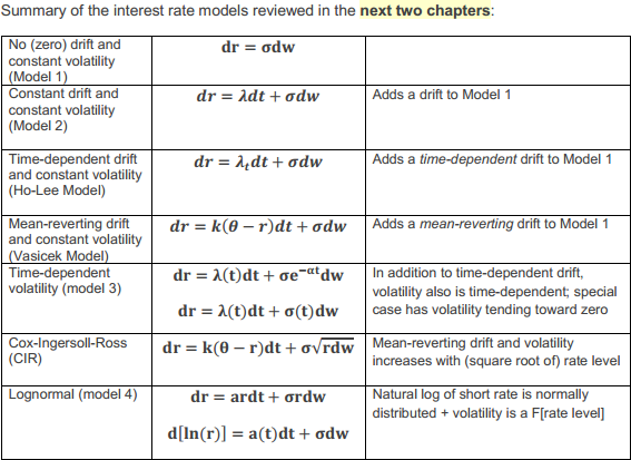Finally, there are two flavors of lognormal model. I hope that is helpful!

 

[brian.field]

This is fantastic! Thank you David!

 

[David Harper CFA FRM]

@brian.field Thank you! FYI, since I had to fix the CIR function I revised the summary table as follows: