You are using an out of date browser. It may not display this or other websites correctly.
You should upgrade or use an alternative browser.
You should upgrade or use an alternative browser.
VaR and ES for Discrete RV
- Thread starter brian.field
- Start date
Great exercise! My opinion is that only the first question has more than one valid, non-esoteric answer
Dowd on VaR in the case of a discrete distribution:
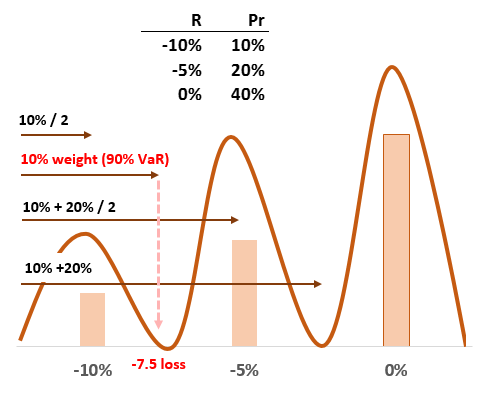
- 90% VaR: According to Dowd, it's arguably -5% (loss of 5%); according to Jorion, it is -10%. Dowd acknowledges the mathematically ambiguity of selecting a VaR when, essentially, the quantile falls exactly between two densities (see quote below). The analogy is HS with, say, n = 1,000; for a 95% VaR, Dowd selects the "less conservative" 51st worst loss and Jorion selects the more conservative (ie, higher VaR) 50th worst loss. Further, in this case, the hybrid approach (to me) fits very well (this is Hull's or Linda Allen's): here, the worst loss observation (-10% loss) is a random variable with its own distributional center (ie, loss of -10%) at the cumulative weight of 10%/2 = 5.0%. In this way: loss at -10% --> weight of 10%/2 = 5.0%; loss at -7.5% = average (-10%, -5%) --> weight of 10%; and loss at -5% --> weight of 20% = 10% + 20%/2. With implied: 95% VaR = -10.0%, 90% VaR = -7.5%, 80% VaR = -5%. In summary, 90% VaR here equals -10% (Jorion), -5% (Dowd) or even -7.5% (L Allen).
- I think Dowd would say the 95% VaR is unambiguously -10%, as the 5% quantile lies unambiguously in the worst probability mass. And to me, that's always the FRM exam answer, too! As above, the only caveat is if we are getting technical-fancy and interpolating due to the assumption that observations are random variables, but that would need to be stated (and it's very unlikely on the exam; the exam has rarely strayed beyond HS)
- The ES is never mathematically ambiguous, as a conditional mean; i.e., both discrete and continuous distributions that meet the probability criteria will always produce means. Re: doesn't the ES need to exceed the VaR? No, this is a common misconception. The ES has no dependence on the VaR. The 90% ES is the average of the 10% tail, full stop. Conveniently, in your case, that's -10%. Notice we don't need to reference any VaR. Good thinking exercises here include: What is the 95% ES? What is the 85% ES?
Dowd on VaR in the case of a discrete distribution:
[footnote 5]: "It is obvious from the figure that the VaR is unambiguously defined when dealing with a continuous P/L distribution. However, the VaR can be ambiguous when the P/L distribution is discontinuous (e.g., as it might be if the P/L distribution is based on historical experience). To see this, suppose there is a gap between the lowest 5% of the probability mass on the left of a figure otherwise similar to Figure 2.4, and the remaining 95% on the right. In this case, the VaR could be the negative of any value between the left-hand side of the 95% mass and the right-hand side of the 5% mass: discontinuities can make the VaR ambiguous. However, in practice, this issue boils down to one of approximation, and won’t make much difference to our results given any reasonable sample size." -- page 27
Last edited:
Thanks David. In your first Dowd Video for Chapter 3, at around the 3 minute 40 second mark, you mention that the ES will always exceed the VaR. (I assumed this was the case as long ast he X% VaR and X% ES are using the same X%)
Hi @brian.field oohhh, sorry, i get you. Yes, that is true, for a given confidence, say C, ES(C) ≥ VaR(C) because the ES is the average of losses that, in this case, exceed the (C) so the ES is taking a weighted average of a set of losses none of which are lower than C! I probably was imprecise: for a given confidence/significance, I should have set the associated ES is greater than or equal to the VaR.
Hi David,
Can you please clarify the bold and underlined portion in your explanations above?
what is Jorion's logic of choosing 90% VaR as -10%?
how do we calculate 90% VaR as - 7.5% as per Linda Allen? Why do we use cumulative weight here?
90% VaR: According to Dowd, it's arguably -5% (loss of 5%); according to Jorion, it is -10%. Dowd acknowledges the mathematically ambiguity of selecting a VaR when, essentially, the quantile falls exactly between two densities (see quote below). The analogy is HS with, say, n = 1,000; for a 95% VaR, Dowd selects the "less conservative" 51st worst loss and Jorion selects the more conservative (ie, higher VaR) 50th worst loss. Further, in this case, the hybrid approach (to me) fits very well (this is Hull's or Linda Allen's): here, the worst loss observation (-10% loss) is a random variable with its own distributional center (ie, loss of -10%) at the cumulative weight of 10%/2 = 5.0%. In this way: loss at -10% --> weight of 10%/2 = 5.0%; loss at -7.5% = average (-10%, -5%) --> weight of 10%; and loss at -5% --> weight of 20% = 10% + 20%/2. With implied: 95% VaR = -10.0%, 90% VaR = -7.5%, 80% VaR = -5%. In summary, 90% VaR here equals -10% (Jorion), -5% (Dowd) or even -7.5% (L Allen).
Regards,
Trilo
Hi @Tril
Linda Allen, Chapter 2 Page 50:
"A minor technical point related to HS is in place here. With 100 observations the first percentile could be thought of as the first observation. However, the observation itself can be thought of as a random event with a probability mass centered where the observation is actually observed, but with 50 percent of the weight to its left and 50 percent to its right. As such, the probability mass we accumulate going from minus infinity to the lowest of 100 observations is only 1/2 percent and not the full 1 percent. According to this argument the first percentile is somewhere in between the lowest and second lowest observation. Figure 2.10 clarifies the point."
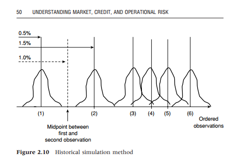
- 90% VaR is an example of when VaR is ambiguous: in a discrete distribution, when the probability falls right "in between" two densities. Here is an analogy (simple HS), say among 100 P/L, the three worst losses are -100, -99, and -98; Jorion here finds the 99% VaR to be -100, but Dowd finds -99 (while Hull/Allen find -99.5). None is wrong. Jorion's logic is defended with something like "1% of the time we expect losses of at least -10%." Dowd's logic would be something like "1% of the time we expect losses worse than -5%."
- It's always a cumulative weight; even in the simple example above (n = 100, with -100, -99, ...), the 95.0% VaR is the loss quantile at the cumulative weight of 5.0%. The Linda Allen/John Hull difference is that--instead of assuming the cumulative weight of 10% (pdf = CDF in the first bin only) aligns with a -10% loss (per the obvious literal reading of Brian's table above), the -10% loss is assumed to be a random variable (observation) with half of its weight to the left (starting at zero) and half of its weight to the right (going to the midpoint of -10% loss and -5% loss which is -7.5% loss, so 10% cumulative probability is associated with loss of -7.5). Further, this implies that the weight associated with -5% loss is the 10% weight (aligning with -7.5 loss) plus one-half the 20.0% weight assigned to -5 loss, such that 20% cumulative probability (i.e., 10% + 20%/2) is associated with the -5.0% loss quantile. See Linda Allen below.
Linda Allen, Chapter 2 Page 50:
"A minor technical point related to HS is in place here. With 100 observations the first percentile could be thought of as the first observation. However, the observation itself can be thought of as a random event with a probability mass centered where the observation is actually observed, but with 50 percent of the weight to its left and 50 percent to its right. As such, the probability mass we accumulate going from minus infinity to the lowest of 100 observations is only 1/2 percent and not the full 1 percent. According to this argument the first percentile is somewhere in between the lowest and second lowest observation. Figure 2.10 clarifies the point."

Last edited:
I just wanted to add an image to clarify the hybrid (ie., Linda Allen above or John Hull) approach, using Brian's data above. Hopefully this makes it easier to see how, for example, we could associate a -7.5% loss (as the midpoint between -10% and -5%) with the 90.0% VaR (i.e., 10% cumulative weight, the second horizontal arrow)

Last edited:
I am wondering how you created that image!!!!
Thanks @brian.field it's just Excel, i've spent too much time in Excel over the years, for years my job was mostly in Excel: the above me literally 5-7 minutes (but the curves are just drawn b/c i was in a hurry). But I'm learning R (rstats) now, which has a steeper learning curve (yikes, actually, I've been practicing R for about two years and I'm only a moderate R coder ...)
I, too, am an excel expert!! Which is why I was wondering  (Since it doesn't seem to me to be entirely straight forward -particularly the curve portion!)
 (Since it doesn't seem to me to be entirely straight forward -particularly the curve portion!)
Ah, cool! I just drew the curves with Insert > Shapes > Curves, here is the XLS if you are interested @ http://trtl.bz/0324-hybrid-var
Thanks!
I just wanted to add an image to clarify the hybrid (ie., Linda Allen above or John Hull) approach, using Brian's data above. Hopefully this makes it easier to see how, for example, we could associate a -7.5% loss (as the midpoint between -10% and -5%) with the 90.0% VaR (i.e., 10% cumulative weight, the second horizontal arrow)

Thanks David! It is very clear now. Need a help on spectral measures concept. Sorry, couldn't find the right forum page, so asking here. Will you please point me to right source in forum discussion/ any other source to have a conceptual understanding of spectral measures?
Regards,
Trilo
Similar threads
- Replies
- 0
- Views
- 292
- Replies
- 0
- Views
- 474
- Replies
- 0
- Views
- 458
- Replies
- 0
- Views
- 463

