YouTube T2-9c Bayes Theorem, Three-state variable

Nicole Seaman

Director of CFA & FRM Operations
Staff member
Subscriber
This explores the answer to Miller's sample question in Chapter 6 of Mathematics and Statistics for Financial Risk Management. There are three types of managers: Out-performers (MO), in-line performers (MI) and under-performers (MU). The prior probability that a manager is an outperformer is 20.0%. But if we observe two years of market beating performance, (aka, evidence), then what is the posterior (updated) probability that the manager is an outperfomer?

Here is David's XLS: https://trtl.bz/220122-bayes-three-states

 
Last edited by a moderator:

Amierul

New Member
Hi @David Harper CFA FRM , can you please help me to answer this question;

1.) Why is it called bayes theorem in --> multiple states?
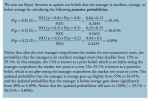
2.) Why the probabilities are presented in different conventions? it is really confusing.

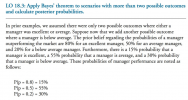
What I meant is this: P(P=0.8)= 15%, P(P=0.5)= 55%, and P(P=0.2)= 30% ?

Given the question below;

Thanks in advance!!

1645695312771.png

1645695344773.png
 

David Harper CFA FRM

David Harper CFA FRM
Subscriber
HI @Amierul

I can drop this into our Bayes learning XLS if you want to see it dynamically illustrated (let me know?), but I don't see unusual conventions here.
  1. It's multi-state because, while you can summarize the typical textbook situation in a 2*2 probability, here you need a 2*3 matrix: two levels of performance (outperformance versus not, O vs O') and three levels of manager talent (excellent, average, and below). The standard setup just needs the negations (i.e., the second outcome can always just be "not the first outcome") so the second state can always be "not the first state," but here you have three categories for one of the dimensions. It's not just a yes/no outcome for both dimensions.
  2. I agree that "P(p = 0.8) = 15%" can be confusing but you can just do this:
Replace "p = 0.8" with "Excellent", replace "p = 0.5" with "Average", and replace "p = 0.2" with "Below". I will go further and just use "E | A | B", then our matrix will just be O | O' versus E | A | B

So the first solution which seeks "P(p = 0.8|O) is just seeking P(Excellent | O) or P(E | O), but the real complication here is that we've observed two consecutive years of outperformance, so we've observed 2O (that's an "O" not a zero 0), so come to think of it, my problem with the notation is that it should read:

P(E | 2O) = P(E ∩ 2O)/P(2O) = P(2O | E)*P(E) / P(2O) = 80%^2 * 15% / 0.2455 = 39.1%

Let me know if that clarifies? Thanks,
 

Amierul

New Member
Hi @David Harper CFA FRM I would really appreciate if you can answer my another concern on the understanding of Bayes Theorem.

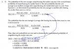
Most of the time, in finding the outperforming probabilities, P(O), I would need to square the conditional probabilities if it is 2 years in a row and multiple it by the uncondional probabilities. For instance, P(O)= (P(O|A))^2*P(A) + (P(O|B))^2*P(B). But in the example below it is really strange that it uses P(A) & P(B) based on the updated belief, where P(A) becomes P(A|O) and P(B) becomes P(B|O).

I dont quite understand in what situation we will use the updated belief or probabilities in finding the unconditonal probabilites of outperforming (line in blue). Can you please help to explain..? tks..


1645984334352.png
1645984346403.png

1645984239905.png
 

David Harper CFA FRM

David Harper CFA FRM
Subscriber
Hi @Amierul It's Sunday and I still have another 8 hour workday so I don't want to get too far into the weeds of some other provider's questions, but briefly: that solution does look correct to me. As before, my only gripe is the notation, where I think, given the question, the notation should read:

P(E | 3O) = ... = 41.956%, and
P(A | 3O) = ... = 58.044%; I do get the same answers

Then the solution is given by:
P(O) = P(O|E)*P(E) + P(O|A)*P(A) = ... = 62.59%; almost exactly the same.

I think I grok your confusion: this is an intermediate/advanced Bayes application, so it is a bit tricky. It's essentially requiring you to solve in two stages:
  1. The first stage is to use Bayes to determine the (posterior) conditional probabilities, P(E | 3O) and P(A | 3O). We are given the priors when we are told the (unconditional) probability of an Excellent manager is 15%. The "evidence" of three consecutive outperforms enables us to update our priors and decide that the posterior probability is 41.96%. The problem could have stopped here, as we've applied Bayes.
  2. But the problem goes further and requires us to treat the above posterior probability "freshly" as a new unconditional probability; i.e., we don't know if this manager is excellent. But we were able to revise a prior with evidence into an updated (posterior) probability that is our "new, better" unconditional. This second step is not Bayes, it is merely a weighted average probability of the to "new" probabilities. I hope that's helpful!
 
Top