R15.P1.T2.DIEBOLD_CH7_Topic: WOLD'S_REPRESENTATION & COVARIANT-STATIONARY

[gargi.adhikari]

In Reference to R15.P1.T2.DIEBOLD_CH7_Topic: WOLD'S_REPRESENTATION & COVARIANT-STATIONARY :-
In Diebold Ch-7: On Pg 20 we have a statement stating the following:
The " Non-Stationary Components " such as "Trends & Seasonality" should be removed from a Time Series to ultimately form a Covariance-Stationary-Series.

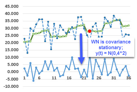
But then On Pg 24: (2nd Screenshot) We have the following statement for Wold's Theorem..
" We really need an appropriate model for “what’s left” after fitting the Trend and Seasonal components; i.e., a model for a Covariance-Stationary Residual
My Question is that, don't we "Remove" the Trend and Seasonal Components and Not "Fit" them into the Model...am I understanding this correctly..? Appreciate and thankful for sharing insights on this.

 

[David Harper CFA FRM]

Hi @gargi.adhikari The summary notes are pretty faithful (literal) to the source Diebold; my feedback to GARP has been that this Diebold is very difficult for candidates because it assigned chapters lack the context of the rest of the book. I think what you are citing here might be merely a case of the language (words) chosen. In both cases, Diebold just means to decompose the series--i.e., parse out the non-stationary components (contributors) such as trend--so that's "what is left over" in the residual component is itself a stationary series.

The time series models are actually pretty fun to play with. I think these both (your citations) are referring to the same idea. To illustrate, I just took the data from my own question 701.1 (original question is here https://forum.bionicturtle.com/thre...-analysis-to-model-seasonality-diebold.10131/ ) which attempts to illustrate a model for Housing Starts. My original model is completely deterministic, but I added another column (another component) which is purely Gaussian White noise and given in excel by a formula I use a lot: =NORM.INV(RAND(),µ, σ). The revised model is plotted below (at least one sample trial). The green is the original housing start model; see how it trends up but also has a seasonal pattern. I added the random white noise, which itself is lower (because it has µ=0) in solid blue; then I simply added it to the time series to produce a new time series that plots with the dotted blue line. Okay, so imagine we started with that series (dotted blue line). It won't itself be covariance stationary; for one reason, it has an upward trend component. However, we could decompose this time series into its three components, such that (stylistically) Housing_starts[time t] = T + S + WN where T = is the (upward) trend, S = the seasonal series and WN = is the random white noise. In my model, the T is simply (T = time * 0.30) which is an dead-simple trend model with slope of 0.30. By doing this, which again is simply decomposing the trend into three additive components, we have effectively "removed" or "parsed" the trend and seasonality such that what is "left over" is the residual white noise, and the white noise is covariance stationary. (this sheet is here https://www.dropbox.com/s/a1ij8ljb20h9t79/1014-house-start-plus-WN.xlsx?dl=0) I hope that's clarifying!