Pritsker (2001) - P/L distribution of VaR and ES

[emilioalzamora1]

Hi David,

I am referring to Dowd's footnote:
'HS fails to take account of useful information from the upper tail of the P/L distribution. If the stock experiences a series of large falls, then a position that was long the market would experience large losses that should show up, albeit later, in HS risk estimates'

Can someone please explain what is meant by 'upper tail of the P/L'? (perhaps incl. a graphic) and why after a large loss does this loss only show after some time has elapsed in HS?

Thank you!

 

[David Harper CFA FRM]

Hi @emilioalzamora1 I'm a huge fan of footnote readers See image below, which is simply a paste of two of Dowd's images. On the left is "unaltered" math which he calls a P/L , wehre losses are negatives and VaR = -q; e.g., 95% VaR = -(-1.65) = 1.65. On the right, losses are positives and this is called L/P. In this way, the "upper tail of the P/L" refers to profits (or gains) which is the side of the distribution that VaR and ES don't directly measure. So hopefully in this context Dowd's first point is self-explanatory: volatility that spikes due to upside jumps (gains) will not translate into either VaR or ES because they measure the other tail. (and it's a short position that would experience loss in this jump). I attached the referenced paper, FYI (relevant text extracted below)

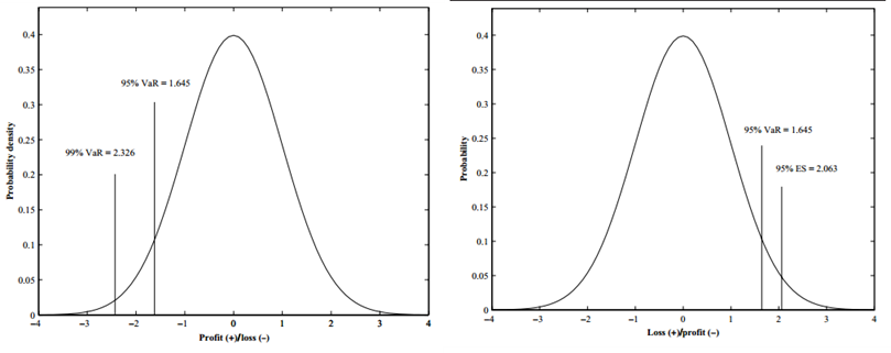
The other point (ie, that extreme losses don't immediately show up) is a weakness of VaR but not ES. Imagine 100 losses, given in L/P format, conveniently ordered from {1, 2, ..., 99, 100}. The 100-day (n=100) 95% ES VaR is 95. Go forward one day with extreme loss of, says, 200. The updated 100-day 95% ES VaR is 96; but that's the same outcome if the new loss were "only" 101. After a few days of extreme losses, the tail will "fill up" and the VaR will jump. I hope that clarifies!

From Page 5 of attached "The Hidden Dangers of Historical Simulation Matthew" (Pritsker, June 19, 2001)

Unfortunately, the BRW method [dharper note: BRW = age-weighted HS or linda allen's hybrid] does not behave nearly as well as the example suggests. To see the problem, instead of considering a portfolio which is long the S&P 500, consider a portfolio which is short the S&P 500. Because the long and short equity positions both involve a “naked” equity exposure, the risk of the two positions should be similar, and should respond similarly to events like a crash. Instead, the crash has very different effects on the BRW estimates of VaR: following the crash the estimated risk of the long portfolio increases very significantly (Figure 1, panels B and C), but the estimated VaR of the short portfolio does not increase at all (Figure 2, panels B and C). The estimated risk of the short portfolio did not increase until the short portfolio experienced significant losses in response to the markets partial recovery in the two days following the crash.

The reason that the BRW method fails to “see” the short portfolio’s increase in risk after the crash is that the BRW method and the historical simulation method are both completely focused on nonparametrically estimating the lower tail of the P&L distribution. Both methods implicitly assume that whatever happens in the upper tail of the distribution, such as a large increase in P&L, contains no information on the lower tail of P&L. This means that large profits are never associated with an increase in the perceived dispersion of returns using either method. In the case of the crash, the short portfolio happened to make a huge amount of money on the day of the crash. As a consequence, the VaR estimates using the BRW and historical simulation methods did not increase.

 

[emilioalzamora1]

Hi David,

many thanks for your insight. As always, great support!

I just want to be clear about your following comment; it does need some more explanation I am afraid:

The other point (ie, that extreme losses don't immediately show up) is a weakness of VaR but not ES. Imagine 100 losses, given in L/P format, conveniently ordered from {1, 2, ..., 99, 100}. The 100-day (n=100) 95% ES is 95. Go forward one day with extreme loss of, says, 200. The updated 100-day 95% ES is 96; but that's the same outcome if the new loss were "only" 101. After a few days of extreme losses, the tail will "fill up" and the VaR will jump. I hope that clarifies!

First, you mention we have 100 losses (for n = 100), so the 95% VaR should be the 6th worst loss: (n x 5% +1) which is (100 x 5% + 1) = 6.
Hence, the 95% VaR is (counting backwards from 100,99,98,97,96,95) = 95.

95% ES should then be the average of the worst 5 losses (100 x 5%) which is: (100+99+98+97+96)/5 = 98.

(So, I don't understand why you get 95% ES = 95?)

You then say 'go forward one day with extreme loss of, says, 200'. Do you mean we now have losses (ordered): 200,100,99,98,97..........or do you mean a window length change?

In case we have losses in the L/P format (ordered from worst downward): 200,100,99,98,97,96,95..........the 95% VaR would simply be (again as given above, the 6th worst loss counting backwards) 96.

And the 95% ES: (200+100+99+98+97)/5 = 118.8

The calculation makes sense to me (and is in line with 'that extreme losses don't immediately show up') if we now compare the 95% ES (changes from 98 to 118.8) while the 95% VaR remains more or less 'unchanged' if you like with the outlier of '200' not accounted for because the 95% VaR only changes from 95 to 96.

Or did I get something totally wrong here?

 

[David Harper CFA FRM]

Hi @emilioalzamora1 Sorry, I should have checked my post more carefully. Above, I did mean VaR not ES. Fixed above , thank you. Exactly as you show, my suspiciously convenient dataset did contemplate:

• as of today, the sorted L/P contain the worst losses of { ... 94, 95, 96, 97, 98, 99, 100} such that the 100-day 95% VaR is the 6th worst (i.e., 95) while the 100-day 95% ES is an average of the five worst (i.e., 98.0 exactly as you show!)
• Then tomorrow a crazy loss of -200 which is +200 in L/P format such that the rolling 100-day (i.e., same window length) worst loss tail now contains { ... 95, 96, 97, 98, 99, 100, 200}; i.e., the 94 "drops out" of the tail and the 200 enters but, keep in mind, these are sorted by loss not time, so the 200 only enters because it falls in the tail. To the first point above, if tomorrow's loss were, say, 50, then the rolling 100-day 95% VaR and 95% ES would be unchanged. But given updated { ... 95, 96, 97, 98, 99, 100, 200}, tomorrows 95% VaR is 96 and 95% ES is 118.8 (exactly as you show, again!). So you have it totally right