Learning objectives: Compare and contrast the age-weighted, the volatility-weighted, the correlation-weighted, and the filtered historical simulation approaches. Identify advantages and disadvantages of non-parametric estimation methods.
Questions:
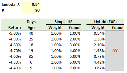
711.1. Bertha the risk analyst has sorted portfolio returns for the last ninety days (K = 90 days) and the worst seven are displayed below. She wants to calculate the age-weighted historical simulation (HS) value at risk (VaR) with 95.0% confidence. Her selected exponential rate of decay, λ - 0.940; e.g., the worst daily loss of -5.0% occurred 40 days ago which is weighted λ^(n-1)*(1-λ)/(1 - λ^K) = 0.940^(40-1)*(1-0.940)/(1-0.940^90) = 0.54%.

There are three ways to retrieve the 95.0% age-weighted historical simulation, but in this case two of them return approximately the same answer. Which of the following pairs is nearest to the 95.0% confident age-weighted historical simulation?
a. 4.50% or 4.55%
b. 4.60% or 4.65%
c. 4.70% or 4.75%
d. 4.80% or 4.75%
711.2. Peter the risk analyst wants to apply the filtered historical simulation approach to his equity portfolio by bootstrapping from a set of standardized returns, where the standardized returns are the result of filtering realized returns with a volatility forecast model. His boss has asked him to incorporate the so-called leverage effect into his model: under this theory a decrease in stock prices automatically implies an increase in firms' leverage (because if market capitalization declines then the ratio of assets to equity must increase) which, in turn, tends to imply an increase in the volatility of equity returns. Therefore, his preference for the (filtering) volatility model is that negative returns (aka, negative shocks) have a more pronounced impact on volatility than positive returns. Which of the following volatility models is best suited for this filtered historical simulation?
a. Exponentially weighted moving average (EWMA) with λ above 0.50
b. GARCH(1,2) model with ω < 0
c. AGARCH σ(n-1)^2 = ω + α*[ε(n-1) + λ]^2*β*σ(n-1)^2 with λ > 0
d. AGARCH σ(n-1)^2 = ω + α*[ε(n-1) + λ]^2*β*σ(n-1)^2 with λ < 0
711.3. Consider the following non-parametric and/or semi-parametric approaches to historical simulation:
I. Basis historical simulation
II. Bootstrapped historical simulation
III. Age-weighted historical simulation
IV. Volatility-weighted historical simulation
V. Correlation-weighted historical simulation
VI. Filtered historical simulation
Which of these above approaches naturally allow us to obtain value at risk (VaR) and expected shortfall (ES) estimates that might EXCEED the maximum loss in our historical dataset?
a. None of them
b. II., III., and IV. only.
c. IV., V., and VI. only
d. All of them
Answers here:
Questions:
711.1. Bertha the risk analyst has sorted portfolio returns for the last ninety days (K = 90 days) and the worst seven are displayed below. She wants to calculate the age-weighted historical simulation (HS) value at risk (VaR) with 95.0% confidence. Her selected exponential rate of decay, λ - 0.940; e.g., the worst daily loss of -5.0% occurred 40 days ago which is weighted λ^(n-1)*(1-λ)/(1 - λ^K) = 0.940^(40-1)*(1-0.940)/(1-0.940^90) = 0.54%.

There are three ways to retrieve the 95.0% age-weighted historical simulation, but in this case two of them return approximately the same answer. Which of the following pairs is nearest to the 95.0% confident age-weighted historical simulation?
a. 4.50% or 4.55%
b. 4.60% or 4.65%
c. 4.70% or 4.75%
d. 4.80% or 4.75%
711.2. Peter the risk analyst wants to apply the filtered historical simulation approach to his equity portfolio by bootstrapping from a set of standardized returns, where the standardized returns are the result of filtering realized returns with a volatility forecast model. His boss has asked him to incorporate the so-called leverage effect into his model: under this theory a decrease in stock prices automatically implies an increase in firms' leverage (because if market capitalization declines then the ratio of assets to equity must increase) which, in turn, tends to imply an increase in the volatility of equity returns. Therefore, his preference for the (filtering) volatility model is that negative returns (aka, negative shocks) have a more pronounced impact on volatility than positive returns. Which of the following volatility models is best suited for this filtered historical simulation?
a. Exponentially weighted moving average (EWMA) with λ above 0.50
b. GARCH(1,2) model with ω < 0
c. AGARCH σ(n-1)^2 = ω + α*[ε(n-1) + λ]^2*β*σ(n-1)^2 with λ > 0
d. AGARCH σ(n-1)^2 = ω + α*[ε(n-1) + λ]^2*β*σ(n-1)^2 with λ < 0
711.3. Consider the following non-parametric and/or semi-parametric approaches to historical simulation:
I. Basis historical simulation
II. Bootstrapped historical simulation
III. Age-weighted historical simulation
IV. Volatility-weighted historical simulation
V. Correlation-weighted historical simulation
VI. Filtered historical simulation
Which of these above approaches naturally allow us to obtain value at risk (VaR) and expected shortfall (ES) estimates that might EXCEED the maximum loss in our historical dataset?
a. None of them
b. II., III., and IV. only.
c. IV., V., and VI. only
d. All of them
Answers here:

