Learning objectives: Describe linear and nonlinear time trends. Explain how to use regression analysis to model seasonality. Describe a random walk and a unit root.
Questions:
21.1.1. The following seasonal dummy model estimates the quarterly growth rate (in percentage terms) of housing starts:

The model's intercept (δ) equals +1.20 and the gamma coefficients are the following: γ(1) = -2.60, γ(2) = +7.90, and γ(3) = +1.80. According to this model, when does the growth rate peak?
a. The peak depends on the year
b. The growth rate peaks at 9.10 in the second quarter
c. The growth rate peaks at 8.30 in the fourth quarter
d. It never peaks because the growth rate has a deterministic, upward trend
21.1.2. Peter wants to model the following AR(2) time series: Y(t) = 0.750*Y(t-1) - 0.1250*T(t-2) + e(t). He wonders if this AR(2) is stationary. He realizes that he can write this as a lag polynomial:
a. This AR(2) is non-stationary and Peter incorrectly factored the polynomial
b. This AR(2) is non-stationary because the sum of the coefficients is less than one
c. This AR(2) is stationary because the sum of the coefficients is less than one
d. This AR(2) is stationary because both roots of the characteristic equation are greater than one
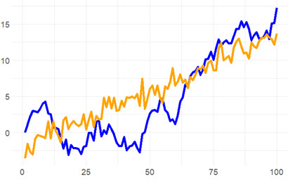
21.1.3. Sally considers two series for her model: a linear trend model (aka, deterministic trend), and a random walk with drift. Each is simulated below (n = 100 steps):

Her two models are given by the following specifications:
a. Sally does not need to do anything because both series are already stationary
b. Sally can detrend the random walk but she should difference the linear trend model if she seeks white noise processes
c. Sally can difference the random walk but she should detrend the linear trend model if she seeks white noise processes
d. Sally wants to estimate the slope coefficients because she can observe that both series already generalize (i.e., are versions of) an MA(1) model where the parameter is the trend's slope
Answers:
Questions:
21.1.1. The following seasonal dummy model estimates the quarterly growth rate (in percentage terms) of housing starts:

The model's intercept (δ) equals +1.20 and the gamma coefficients are the following: γ(1) = -2.60, γ(2) = +7.90, and γ(3) = +1.80. According to this model, when does the growth rate peak?
a. The peak depends on the year
b. The growth rate peaks at 9.10 in the second quarter
c. The growth rate peaks at 8.30 in the fourth quarter
d. It never peaks because the growth rate has a deterministic, upward trend
21.1.2. Peter wants to model the following AR(2) time series: Y(t) = 0.750*Y(t-1) - 0.1250*T(t-2) + e(t). He wonders if this AR(2) is stationary. He realizes that he can write this as a lag polynomial:
- Y(t) = 0.750*L - 0.1250*L^2 + ε(t); first he expresses the model with lag operators
- (1 - 0.750*L + 0.1250*L^2)*Y(t) =ε(t); then he isolates the lag polynomial
- (1 - 0.50*L)(1 - 0.250*L)*Y(t) = ε(t); finally, he factors the polynomial
a. This AR(2) is non-stationary and Peter incorrectly factored the polynomial
b. This AR(2) is non-stationary because the sum of the coefficients is less than one
c. This AR(2) is stationary because the sum of the coefficients is less than one
d. This AR(2) is stationary because both roots of the characteristic equation are greater than one
21.1.3. Sally considers two series for her model: a linear trend model (aka, deterministic trend), and a random walk with drift. Each is simulated below (n = 100 steps):

Her two models are given by the following specifications:
- Y(t) = δ(0) + δ(1)*t + ε(t), and
- Y(t) = δ(0) + Y(t-1) + ε(t).
a. Sally does not need to do anything because both series are already stationary
b. Sally can detrend the random walk but she should difference the linear trend model if she seeks white noise processes
c. Sally can difference the random walk but she should detrend the linear trend model if she seeks white noise processes
d. Sally wants to estimate the slope coefficients because she can observe that both series already generalize (i.e., are versions of) an MA(1) model where the parameter is the trend's slope
Answers:
Last edited:
