Learning objectives: Define covariance and explain what it measures. Explain the relationship between the covariance and correlation of two random variables and how these are related to the independence of the two variables. Explain the effects of applying linear transformations on the covariance and correlation between two random variables.
Questions:
20.9.1. Over the previous six months, two assets generated the monthly returns displayed below under columns X(i) and Y(i). The third and fourth columns display the squared difference-from-average-returns that inform the univariate variance; the fifth column shows the associated cross-product that informs their covariance.

Because this is a very small sample, we want to retrieve unbiased sample moments. What are, respectively, the unbiased sample variances of the two variables and their sample covariance?
a. The unbiased sample variances, σ^2(X) = 2.16 and σ^2(Y) = 2.50 and sample covariance σ(X,Y) = 3.67
b. The unbiased sample variances, σ^2(X) = 4.67 and σ^2(Y) = 6.25 and sample covariance σ(X,Y) = 3.67
c. The unbiased sample variances, σ^2(X) = 4.67 and σ^2(Y) = 6.25 and sample covariance σ(X,Y) = 4.40
d. The unbiased sample variances, σ^2(X) = 5.60 and σ^2(Y) = 7.50 and sample covariance σ(X,Y) = 4.40
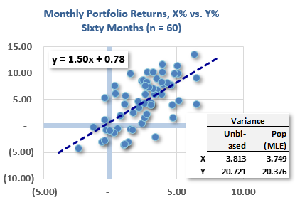
20.9.2. The scatterplot below plots sixty pairwise monthly returns over the last five years; each dot represents the return of Y (on the y-axis) and the return of X (on the x-axis) in a given month. Also shown is the ordinary least squares (OLS) regression line generated by Excel: Y = 1.50*X + 0.78. Finally, the univariate variances for each series are shown.

Which of the following is nearest to the correlation between X and Y? (Bonus question: if we flipped the axes, then what is the correlation?)
a. 0.28
b. 0.41
c. 0.64
d. 1.50
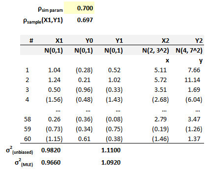
20.9.3. Below is a simulation with a correlation input parameter, ρ(sim param), of 0.70. The simulation has 60 rows (one per month) but the bulk of the middle rows are not displayed. The first two columns, X1 and Y0, are generated by Excel's NORM.S.INV(RAND()); this generates a random standard normal deviate (aka, quantile) such that we expect approximately 68% of the values to fall between (-1.0, 1.0) and 95% to fall between (-2.0, 2.0). The next column, Y1, transforms Y0 in order to generate a random standard normal deviate, Y1, that is correlated to X1. Thus X1 and Y1 are both random standard normal deviates but they are correlated. The ρ(sample) of 0.697 refers to the actual sample correlation: as itself a random variable with an expected value of 0.70, it is very near to the 0.70 but will fluctuate per each simulation. Finally, X2 and Y2 apply a linear transformation, respectively, to X1 and Y1. Specifically, as X1 is a random N(0, 1), X2 has a mean of 2 and a variance of 3^2 or 9; Y2 has a mean of 4 and a variance of 7^2 or 49.

Let us here temporarily refer to the unbiased standard deviation as the square root of the unbiased variance (although this is imprecise). In regard to these linearly transformed X2 and Y2, what are their unbiased standard deviations, and what is their correlation, ρ(X2,Y2)?
a. σ(X2) = 1.00, σ(Y2) = 1.00 and ρ(X2, Y2) = 0.700
b. σ(X2) = 2.97, σ(Y2) = 7.37 and ρ(X2, Y2) = 0.697
c. σ(X2) = 3.00, σ(Y2) = 7.00 and ρ(X2, Y2) = 0.700
d. σ(X2) = 8.84, σ(Y2) = 54.39 and ρ(X2, Y2) = 0.6.97
Answers here:
Questions:
20.9.1. Over the previous six months, two assets generated the monthly returns displayed below under columns X(i) and Y(i). The third and fourth columns display the squared difference-from-average-returns that inform the univariate variance; the fifth column shows the associated cross-product that informs their covariance.

Because this is a very small sample, we want to retrieve unbiased sample moments. What are, respectively, the unbiased sample variances of the two variables and their sample covariance?
a. The unbiased sample variances, σ^2(X) = 2.16 and σ^2(Y) = 2.50 and sample covariance σ(X,Y) = 3.67
b. The unbiased sample variances, σ^2(X) = 4.67 and σ^2(Y) = 6.25 and sample covariance σ(X,Y) = 3.67
c. The unbiased sample variances, σ^2(X) = 4.67 and σ^2(Y) = 6.25 and sample covariance σ(X,Y) = 4.40
d. The unbiased sample variances, σ^2(X) = 5.60 and σ^2(Y) = 7.50 and sample covariance σ(X,Y) = 4.40
20.9.2. The scatterplot below plots sixty pairwise monthly returns over the last five years; each dot represents the return of Y (on the y-axis) and the return of X (on the x-axis) in a given month. Also shown is the ordinary least squares (OLS) regression line generated by Excel: Y = 1.50*X + 0.78. Finally, the univariate variances for each series are shown.

Which of the following is nearest to the correlation between X and Y? (Bonus question: if we flipped the axes, then what is the correlation?)
a. 0.28
b. 0.41
c. 0.64
d. 1.50
20.9.3. Below is a simulation with a correlation input parameter, ρ(sim param), of 0.70. The simulation has 60 rows (one per month) but the bulk of the middle rows are not displayed. The first two columns, X1 and Y0, are generated by Excel's NORM.S.INV(RAND()); this generates a random standard normal deviate (aka, quantile) such that we expect approximately 68% of the values to fall between (-1.0, 1.0) and 95% to fall between (-2.0, 2.0). The next column, Y1, transforms Y0 in order to generate a random standard normal deviate, Y1, that is correlated to X1. Thus X1 and Y1 are both random standard normal deviates but they are correlated. The ρ(sample) of 0.697 refers to the actual sample correlation: as itself a random variable with an expected value of 0.70, it is very near to the 0.70 but will fluctuate per each simulation. Finally, X2 and Y2 apply a linear transformation, respectively, to X1 and Y1. Specifically, as X1 is a random N(0, 1), X2 has a mean of 2 and a variance of 3^2 or 9; Y2 has a mean of 4 and a variance of 7^2 or 49.

Let us here temporarily refer to the unbiased standard deviation as the square root of the unbiased variance (although this is imprecise). In regard to these linearly transformed X2 and Y2, what are their unbiased standard deviations, and what is their correlation, ρ(X2,Y2)?
a. σ(X2) = 1.00, σ(Y2) = 1.00 and ρ(X2, Y2) = 0.700
b. σ(X2) = 2.97, σ(Y2) = 7.37 and ρ(X2, Y2) = 0.697
c. σ(X2) = 3.00, σ(Y2) = 7.00 and ρ(X2, Y2) = 0.700
d. σ(X2) = 8.84, σ(Y2) = 54.39 and ρ(X2, Y2) = 0.6.97
Answers here:
