Learning objectives: Calculate the probability of an event for a discrete probability function. Define and calculate a conditional probability. Distinguish between conditional and unconditional probabilities. Explain and apply Bayes’ rule.
Questions:
20.2.1. The probability graph below illustrates event A (the yellow rectangle) and event B (the blue rectangle). The unconditional probability of event A is 50.0% and the unconditional probability of event B is 44.0%; i.e., Pr(A) = 50.0% and Pr(B) = 44.0%. Their overlap is graphed by the green rectangle such that Pr(A ∩ B) = 27.0%. The orange rectangle conditions on the event C. For example, conditional on event C, there is a 50.0% probability that event A occurs, Pr(A | C) = 50.0%.

Which of the following is TRUE about, respectively, the unconditional and conditional relationship between events A and B?
a. A and B are unconditionally dependent but conditionally (on event C) independent
b. A and B are unconditionally dependent and also conditionally (on event C) dependent
c. A and B are unconditionally independent but conditionally (on event C) dependent
d. A and B are unconditionally independent and also conditionally (on event C) independent
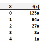
20.2.2. Rebecca is a risk analyst who wants to characterize the loss frequency distribution of a certain minor operational process during each day. On most days, there is no loss event; i.e. Pr(X = 0) > 50.0%. On days when there is at least one loss, there occurs either one, two, three, or four loss events. For this process, she likes the shape of the Poisson distribution with a low mean (e.g., lambda = 1) but the problem is that the Poisson has a long, thin right tail. However, given her frequency outcome is finite, Rebecca prefers a domain limited to only five outcomes including zero: X = {0, 1, 2, 3, or 4}, but X cannot be five or more. She settles on an elegant formula to express the density probability as a function of a constant. Her function is Pr(X = x) = (5-x)^3*a, where (a) is a constant, over the domain mentioned. Specifically Pr(X = 0) = 125*a, Pr(X = 1) = 64*a, and so on.
Basically, this assigns the lowest probability (a) to an outcome of four. An outcome of three is eight times (8a) more likely than an outcome of four. An outcome of two is 27 times more likely (27a) than an outcome of four, an outcome of one is 64 times more likely (64a) than a four, and an outcome of zero is 125 times more likely (125a) than an outcome of four. This allows her to fit her sample database by characterizing the distribution of outcomes in relative terms; i.e., relative to an outcome of four which is the least likely. Specifically, it reflects her want of a distribution under which a zero or one occurs more than 80.0% of the time, yet in rare cases the outcome can be as much as four. Unlike the Poisson, it has no tail beyond an outcome of four. Her probability mass distribution looks like the following:

What is the probability that X will be at least two, Pr(X≥2), which in this case of a discrete distribution is the same as Pr(X > 1)?
a. 2.78%
b. 9.50%
c. 16.00%
d. 36.00%
20.2.3. Among a set of filtered stocks, a stock screener assigns stocks to one of three style categories: value, quality, or momentum. At the end of each month, the stock's performance is compared to the S&P such that it either beats or does not beat the index The prior beliefs (aka, unconditional probabilities) are the following: Pr(Style = Value) = 15.0%, Pr(Style = Quality) = 30.0%, and Pr(Style = Momentum) = 55.0%.
Bonus question: if we observe the stock beats the index two months in a row, what is the probability it is a momentum stock; i.e., what is Pr(Momentum | Two consecutive Beats)?
a. 39.6%
b. 55.0%
c. 64.7%
d. 83.3%
Answers here:
Questions:
20.2.1. The probability graph below illustrates event A (the yellow rectangle) and event B (the blue rectangle). The unconditional probability of event A is 50.0% and the unconditional probability of event B is 44.0%; i.e., Pr(A) = 50.0% and Pr(B) = 44.0%. Their overlap is graphed by the green rectangle such that Pr(A ∩ B) = 27.0%. The orange rectangle conditions on the event C. For example, conditional on event C, there is a 50.0% probability that event A occurs, Pr(A | C) = 50.0%.

Which of the following is TRUE about, respectively, the unconditional and conditional relationship between events A and B?
a. A and B are unconditionally dependent but conditionally (on event C) independent
b. A and B are unconditionally dependent and also conditionally (on event C) dependent
c. A and B are unconditionally independent but conditionally (on event C) dependent
d. A and B are unconditionally independent and also conditionally (on event C) independent
20.2.2. Rebecca is a risk analyst who wants to characterize the loss frequency distribution of a certain minor operational process during each day. On most days, there is no loss event; i.e. Pr(X = 0) > 50.0%. On days when there is at least one loss, there occurs either one, two, three, or four loss events. For this process, she likes the shape of the Poisson distribution with a low mean (e.g., lambda = 1) but the problem is that the Poisson has a long, thin right tail. However, given her frequency outcome is finite, Rebecca prefers a domain limited to only five outcomes including zero: X = {0, 1, 2, 3, or 4}, but X cannot be five or more. She settles on an elegant formula to express the density probability as a function of a constant. Her function is Pr(X = x) = (5-x)^3*a, where (a) is a constant, over the domain mentioned. Specifically Pr(X = 0) = 125*a, Pr(X = 1) = 64*a, and so on.
Basically, this assigns the lowest probability (a) to an outcome of four. An outcome of three is eight times (8a) more likely than an outcome of four. An outcome of two is 27 times more likely (27a) than an outcome of four, an outcome of one is 64 times more likely (64a) than a four, and an outcome of zero is 125 times more likely (125a) than an outcome of four. This allows her to fit her sample database by characterizing the distribution of outcomes in relative terms; i.e., relative to an outcome of four which is the least likely. Specifically, it reflects her want of a distribution under which a zero or one occurs more than 80.0% of the time, yet in rare cases the outcome can be as much as four. Unlike the Poisson, it has no tail beyond an outcome of four. Her probability mass distribution looks like the following:

What is the probability that X will be at least two, Pr(X≥2), which in this case of a discrete distribution is the same as Pr(X > 1)?
a. 2.78%
b. 9.50%
c. 16.00%
d. 36.00%
20.2.3. Among a set of filtered stocks, a stock screener assigns stocks to one of three style categories: value, quality, or momentum. At the end of each month, the stock's performance is compared to the S&P such that it either beats or does not beat the index The prior beliefs (aka, unconditional probabilities) are the following: Pr(Style = Value) = 15.0%, Pr(Style = Quality) = 30.0%, and Pr(Style = Momentum) = 55.0%.
- Pr(Beat | Value) = 40.0%
- Pr(Beat | Quality) = 60.0%
- Pr(Beat | Momentum ) = 80.0%
Bonus question: if we observe the stock beats the index two months in a row, what is the probability it is a momentum stock; i.e., what is Pr(Momentum | Two consecutive Beats)?
a. 39.6%
b. 55.0%
c. 64.7%
d. 83.3%
Answers here:
Last edited by a moderator:
