Learning objectives: Explain how to test whether a regression is affected by heteroskedasticity. Describe approaches to using heteroskedastic data. Characterize multicollinearity and its consequences; distinguish between multicollinearity and perfect collinearity. Describe the consequences of excluding a relevant explanatory variable from a model and contrast those with the consequences of including an irrelevant regressor.
Questions:
20.19.1. Jane manages a market-neutral equity fund for her investment management firm. The fund's market-neutral style implies (we will assume) that the fund's beta with respect to the market's excess return is zero. However, the fund does seek exposure to other factors. The size factor captures the excess return of small-capitalization stocks (SMB = "small minus big"). Jane tests her portfolio's exposure to the size factor by regressing the portfolio's excess return against the size factor returns. Her regression takes the form PORTFOLIO(i) = α + β1×SMB(i) + ε(i). The results of this single-variable (aka, simple) regression are displayed below.
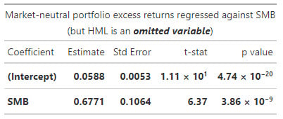
In this simple regression, we can observe that SMB's coefficient is 0.6771 and significant. Jane is concerned that this simple regression might suffer from omitted variable bias. Specifically, she thinks the value factor has been omitted. The value factor captures the excess returns of value stocks (HML = "high book-to-market minus low book-to-market")'. She confirms that the omitted variable, HML, is associated with her response variable. Further, the omitted variable, HML, is correlated to SMB. The correlation between HML and SMB is 0.30. Further, the volatility of HML and SMB happen to be identical; i.e., σ(MHL) = σ(SMB).
Consequently (to remedy the omitted variable problem), Jane runs a multivariate regression that includes both explanatory variables, SMB and HML. In this regression, HML's beta coefficient is 0.7240 such that the new term is β2×HML(i) = 0.7240×HML(i). Which of the following is nearest to the revised SMB coefficient; i.e., what is the revised β1?
a. 0.230
b. 0.460
c. 0.677
d. 1.253
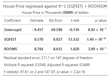
20.19.2. Josh regressed house prices (as the response or dependent variable) against two explanatory variables: square footage (SQFEET) and the number of rooms in the house (ROOMS). The dependent variable, PRICE, is expressed in thousands of dollars ($000); e.g., the average PRICE is $728.283 because the average house price in the sample of 150 houses is $728,283. The units of SQFEET are unadjusted units; e.g., the average SQFEET in the sample is 1,893 ft^2. The variable ROOMS is equal to the sum of the number of bedrooms and bathrooms; because much of the sample is 2- and 3-bedroom houses with 2 baths, the average of ROOM is 4.35. Josh's regression results are displayed below.
Josh is concerned that the data might not be homoscedastic. He decides to conduct a White test for heteroskedasticity. In this test, he regresses the squared residuals against each of the explanatory variables and the cross-product of the explanatory variables (including the product of each variable with itself). The results of this regression are displayed below.
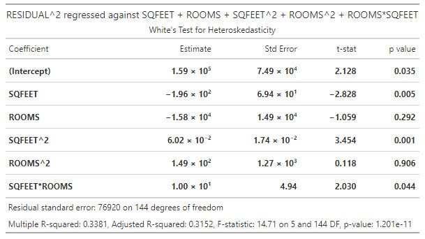
Is the data heteroskedastic?
a. No, the data is probably homoskedastic because all coefficients are highly significant
b. No, the data is probably homoskedastic because the F-statistic does not imply the rejection of the null hypothesis
c. Yes, the data is probably heteroskedastic because the m-fold cross-validation failed
d. Yes, the data is probably heteroskedastic because the residual variance has some dependence on SQFEET
20.19.3. Emily works for an insurance company and she has regressed medical costs (aka, the response or dependent variable) for a sample of patients against three independent variables: AGE, BMI, and CHARITY. The sample's average age is 38.5 years. Body mass index (BMI) is mass divided by height squared and the sample's average BMI is 22.24 kg/m^2. CHARITY is the dollar amount of charitable spending in the last year; the sample average is $511.66 donated to charity in the last year. Emily's regression results are displayed below.
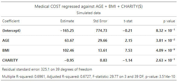
Emily wonders if the data exhibits multicollinearity. In order to test for multicollinearity, she conducts three additional regressions. She regresses each of the explanatory variables against the other two explanatory variables. Below are summarized the R-squared (R^2) values for each of those regressions:
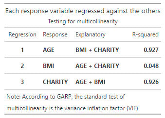
Does Emily's data contain multicollinearity?
a. No, because none of the variance inflation factors (VIFs) are excessive
b. No, because all estimates are significant and the Adjusted R-squared is above 0.50
c. Yes, because two of the variance inflation factors (VIFs) are excessive
d. Yes, because the R-squared of BMI is less than 5.0%
Answers here:
Questions:
20.19.1. Jane manages a market-neutral equity fund for her investment management firm. The fund's market-neutral style implies (we will assume) that the fund's beta with respect to the market's excess return is zero. However, the fund does seek exposure to other factors. The size factor captures the excess return of small-capitalization stocks (SMB = "small minus big"). Jane tests her portfolio's exposure to the size factor by regressing the portfolio's excess return against the size factor returns. Her regression takes the form PORTFOLIO(i) = α + β1×SMB(i) + ε(i). The results of this single-variable (aka, simple) regression are displayed below.
In this simple regression, we can observe that SMB's coefficient is 0.6771 and significant. Jane is concerned that this simple regression might suffer from omitted variable bias. Specifically, she thinks the value factor has been omitted. The value factor captures the excess returns of value stocks (HML = "high book-to-market minus low book-to-market")'. She confirms that the omitted variable, HML, is associated with her response variable. Further, the omitted variable, HML, is correlated to SMB. The correlation between HML and SMB is 0.30. Further, the volatility of HML and SMB happen to be identical; i.e., σ(MHL) = σ(SMB).
Consequently (to remedy the omitted variable problem), Jane runs a multivariate regression that includes both explanatory variables, SMB and HML. In this regression, HML's beta coefficient is 0.7240 such that the new term is β2×HML(i) = 0.7240×HML(i). Which of the following is nearest to the revised SMB coefficient; i.e., what is the revised β1?
a. 0.230
b. 0.460
c. 0.677
d. 1.253
20.19.2. Josh regressed house prices (as the response or dependent variable) against two explanatory variables: square footage (SQFEET) and the number of rooms in the house (ROOMS). The dependent variable, PRICE, is expressed in thousands of dollars ($000); e.g., the average PRICE is $728.283 because the average house price in the sample of 150 houses is $728,283. The units of SQFEET are unadjusted units; e.g., the average SQFEET in the sample is 1,893 ft^2. The variable ROOMS is equal to the sum of the number of bedrooms and bathrooms; because much of the sample is 2- and 3-bedroom houses with 2 baths, the average of ROOM is 4.35. Josh's regression results are displayed below.
Josh is concerned that the data might not be homoscedastic. He decides to conduct a White test for heteroskedasticity. In this test, he regresses the squared residuals against each of the explanatory variables and the cross-product of the explanatory variables (including the product of each variable with itself). The results of this regression are displayed below.
Is the data heteroskedastic?
a. No, the data is probably homoskedastic because all coefficients are highly significant
b. No, the data is probably homoskedastic because the F-statistic does not imply the rejection of the null hypothesis
c. Yes, the data is probably heteroskedastic because the m-fold cross-validation failed
d. Yes, the data is probably heteroskedastic because the residual variance has some dependence on SQFEET
20.19.3. Emily works for an insurance company and she has regressed medical costs (aka, the response or dependent variable) for a sample of patients against three independent variables: AGE, BMI, and CHARITY. The sample's average age is 38.5 years. Body mass index (BMI) is mass divided by height squared and the sample's average BMI is 22.24 kg/m^2. CHARITY is the dollar amount of charitable spending in the last year; the sample average is $511.66 donated to charity in the last year. Emily's regression results are displayed below.
Emily wonders if the data exhibits multicollinearity. In order to test for multicollinearity, she conducts three additional regressions. She regresses each of the explanatory variables against the other two explanatory variables. Below are summarized the R-squared (R^2) values for each of those regressions:
Does Emily's data contain multicollinearity?
a. No, because none of the variance inflation factors (VIFs) are excessive
b. No, because all estimates are significant and the Adjusted R-squared is above 0.50
c. Yes, because two of the variance inflation factors (VIFs) are excessive
d. Yes, because the R-squared of BMI is less than 5.0%
Answers here:
Last edited by a moderator: