Learning objectives: Distinguish between the relative assumptions of single and multiple regression. Interpret regression coefficients in a multiple regression. Interpret goodness of fit measures for single and multiple regressions, including R2 and adjusted-R2. Construct, apply and interpret joint hypothesis tests and confidence intervals for multiple coefficients in a regression.
Questions:
20.18.1. Sally is a portfolio manager at an investment management firm. She wants to test her primary equity portfolio's reaction to the factors in the Fama-French three-factor model. She collected excess returns (i.e., net of the riskfree rate) over the last eight years, so that the sample size, n = 96 months. The response (aka, explained, dependent) variable is the portfolio's excess return. The three explanatory variables are the market factor (MKT), the size factor (SMB), and the value factor (HML). The size factor captures the excess return of small capitalization stocks (SMB = "small minus big") and the value factor captures the excess returns of value stocks (HML = "high book-to-market minus low book-to-market")'. Sally's regression results are displayed below.
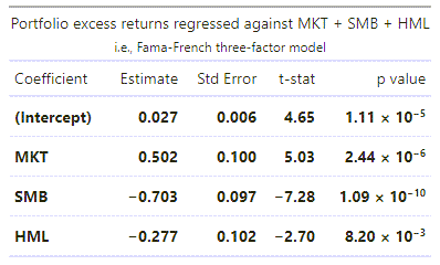
Which of the following descriptions of her portfolio is the most accurate?
a. Her small capitalization, value-oriented low-beta portfolio has not generated alpha
b. Her large capitalization, growth-oriented high-beta portfolio has not generated alpha
c. Her large capitalization, growth-oriented low-beta portfolio has generated significantly positive alpha
d. Her small capitalization, value-oriented high-beta portfolio has generated significantly positive alpha
20.18.2. Derek regressed house prices (as the response or dependent variable) against three explanatory variables: square footage (SQFEET), number of rooms in the house (ROOMS), and age of the house (AGE). The dependent variable, PRICE, is expressed in thousands of dollars ($000); e.g., the average PRICE is $386.051 because the average house price in the sample of 96 houses is $386,051. The units of SQFEET are unadjusted units; e.g., the average SQFEET in the sample is 1,203 ft^2. The variable ROOMS is equal to the sum of the number of bedrooms and bathrooms; because much of the sample is 2- and 3-bedroom houses with 2 baths, the average of ROOM is 4.55. Finally, AGE is given in years where the average AGE in the sample is 14.77 years. Derek's regression results are displayed below.
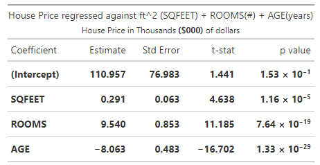
Each of the following statements is true about these regression results EXCEPT which is false?
a. Older houses have lower prices on average
b. The 98.0% confidence interval (CI) for the AGE coefficient is (5.7, 10.4)
c. The 90.0% confidence interval (CI) for the ROOMS coefficient is (8.1, 10.9)
d. An additional (+) 100 square feet (ft^2) is associated with an expected increase of ~ $29,100 in the price of the house
20.18.3. Mary works for an insurance company and she has regressed medical costs (aka, the response or dependent variable) for a sample of patients against four independent variables: AGE, BMI, SMOKER, and CHARITY. The sample's average age is 38.51 years. Body mass index (BMI) is mass divided by height squared and the sample's average BMI is 22.16. SMOKER is a dummy variable where zero indicates a non-smoker and 1 indicates a smoker; the sample's average SMOKER value is 0.163 which indicates that 16.3% of the sample are smokers. CHARITY is the dollar amount of charitable spending in the last year; the sample average is $490.70 donated to charity in the last year. Mary's regression results are displayed below.
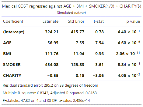
Each of the following statements is true about these regression results EXCEPT which is false?
a. The sample size is 43 patients
b. Mary can reject a null hypothesis that all explanatory variables (jointly) have zero coefficients
c. Mary can infer that patient medical cost is positively associated with each of AGE, BMI, and, on average, is greater for a smoker
d. Mary should suspect problematic multicollinearity because the intercept is suspiciously negative and the adjusted R-squared is too near to the unadjusted R-squared
Answers here:
Questions:
20.18.1. Sally is a portfolio manager at an investment management firm. She wants to test her primary equity portfolio's reaction to the factors in the Fama-French three-factor model. She collected excess returns (i.e., net of the riskfree rate) over the last eight years, so that the sample size, n = 96 months. The response (aka, explained, dependent) variable is the portfolio's excess return. The three explanatory variables are the market factor (MKT), the size factor (SMB), and the value factor (HML). The size factor captures the excess return of small capitalization stocks (SMB = "small minus big") and the value factor captures the excess returns of value stocks (HML = "high book-to-market minus low book-to-market")'. Sally's regression results are displayed below.

Which of the following descriptions of her portfolio is the most accurate?
a. Her small capitalization, value-oriented low-beta portfolio has not generated alpha
b. Her large capitalization, growth-oriented high-beta portfolio has not generated alpha
c. Her large capitalization, growth-oriented low-beta portfolio has generated significantly positive alpha
d. Her small capitalization, value-oriented high-beta portfolio has generated significantly positive alpha
20.18.2. Derek regressed house prices (as the response or dependent variable) against three explanatory variables: square footage (SQFEET), number of rooms in the house (ROOMS), and age of the house (AGE). The dependent variable, PRICE, is expressed in thousands of dollars ($000); e.g., the average PRICE is $386.051 because the average house price in the sample of 96 houses is $386,051. The units of SQFEET are unadjusted units; e.g., the average SQFEET in the sample is 1,203 ft^2. The variable ROOMS is equal to the sum of the number of bedrooms and bathrooms; because much of the sample is 2- and 3-bedroom houses with 2 baths, the average of ROOM is 4.55. Finally, AGE is given in years where the average AGE in the sample is 14.77 years. Derek's regression results are displayed below.

Each of the following statements is true about these regression results EXCEPT which is false?
a. Older houses have lower prices on average
b. The 98.0% confidence interval (CI) for the AGE coefficient is (5.7, 10.4)
c. The 90.0% confidence interval (CI) for the ROOMS coefficient is (8.1, 10.9)
d. An additional (+) 100 square feet (ft^2) is associated with an expected increase of ~ $29,100 in the price of the house
20.18.3. Mary works for an insurance company and she has regressed medical costs (aka, the response or dependent variable) for a sample of patients against four independent variables: AGE, BMI, SMOKER, and CHARITY. The sample's average age is 38.51 years. Body mass index (BMI) is mass divided by height squared and the sample's average BMI is 22.16. SMOKER is a dummy variable where zero indicates a non-smoker and 1 indicates a smoker; the sample's average SMOKER value is 0.163 which indicates that 16.3% of the sample are smokers. CHARITY is the dollar amount of charitable spending in the last year; the sample average is $490.70 donated to charity in the last year. Mary's regression results are displayed below.

Each of the following statements is true about these regression results EXCEPT which is false?
a. The sample size is 43 patients
b. Mary can reject a null hypothesis that all explanatory variables (jointly) have zero coefficients
c. Mary can infer that patient medical cost is positively associated with each of AGE, BMI, and, on average, is greater for a smoker
d. Mary should suspect problematic multicollinearity because the intercept is suspiciously negative and the adjusted R-squared is too near to the unadjusted R-squared
Answers here:
Last edited by a moderator:
