FRM P1 > T2 > StockWatson: Linear Regression (EDA)
Econometrics has always been a backbone topic in the FRM. Subsequent to the exam's P1/P2 split, the 2009 assignment was Gujarati's Essentials of Econometrics (3rd Edition), which remains one of my favorite references due to its clarity and technical precision. Currently, math/statistics are assigned to Miller and linear regression is assigned to Stock & Watson (S&W). In my opinion, S&W is adequate (some of the technical explanations are confusing) while the key drawback is the lack of easily accessible code-based examples/applications; the reality is that we want to understand the application of regression in a modern code-based context. Because that's the realistic context. You can read about regression for many hours, but you won't really understand it until you engage with it code-wise. I prefer R (#rstats) for this but of course Excel is a great OLS regression tool (I believe S&W provides the native datasets for EViews applications--which I did use years ago; see their companion site at http://media.pearsoncmg.com/ph/bp/bridgepages/teamsite/stock_watson/ -- but personally, given the dramatic uptake in the popularity of #rstats, I don't see a reason to invest in EViews learning. I think you are wiser to invest in #rstats learning, but opinions vary).
Our learning spreadsheet (located here in the Study Planner) replicates most of the quantitative concepts in S&W. A helpful aspect of S&W's regression review is the continuity of their using a single dataset as they transition from univariate to multivariate regression. In this brief post I just want to introduce the first three sheets in the workbook.
The first three sheets in the workbook are:
") We might save ourselves some time if the picture reveals something interesting! So here is that picture .... the first thing that jumps out for me is "I'm not sure I see any linear relationship, it sort of looks like a cloud."
We might save ourselves some time if the picture reveals something interesting! So here is that picture .... the first thing that jumps out for me is "I'm not sure I see any linear relationship, it sort of looks like a cloud."
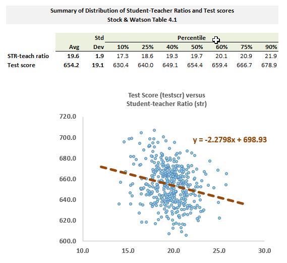
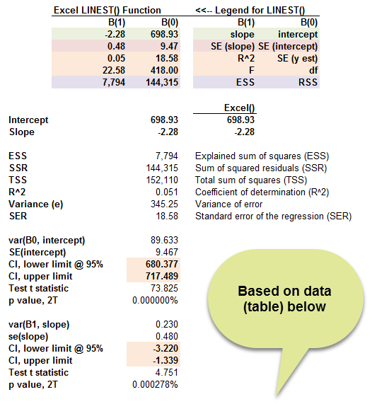
Nevertheless, we can summon an OLS regression line through the data points. Where did the regression results come from? Excel has OLS regression built-in via its highly capable LINEST() array function, but the second sheet (called "0-SW-data-pre-process", the top panel screenshot is below) performs the complete manual estimation of the OLS regression line (I added confidence intervals around the coefficients).
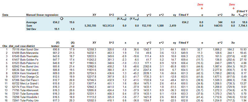
These regression statistics are generated from simple aggregate statistics of the data (see below). For those who really want to explore, this can be interesting. For example, we can see how the mean value of the errors (aka, residuals) is always zero; and, surprisingly, how the summation of [the product of each independent variable and its own residual] is necessarily zero, which confirms the assumption that the residuals are uncorrelated with the independent variables. Mathematically (and visually) there are so many different ways to select a line that draws through the dataset; the OLS regression line is but one choice and it makes interesting assumptions! If you do not want to take the time to explore the manual computation of the linear regression, then consider at least taking a look at Excel's LINEST() array function.
Just to wrap up this post, here are the things that I find interesting/helpful from the OLS regression analysis:
Today I just wanted to introduce the first three sheets in this learning workbook ... on the next post, I will look at the SRF versus the PRF.
Econometrics has always been a backbone topic in the FRM. Subsequent to the exam's P1/P2 split, the 2009 assignment was Gujarati's Essentials of Econometrics (3rd Edition), which remains one of my favorite references due to its clarity and technical precision. Currently, math/statistics are assigned to Miller and linear regression is assigned to Stock & Watson (S&W). In my opinion, S&W is adequate (some of the technical explanations are confusing) while the key drawback is the lack of easily accessible code-based examples/applications; the reality is that we want to understand the application of regression in a modern code-based context. Because that's the realistic context. You can read about regression for many hours, but you won't really understand it until you engage with it code-wise. I prefer R (#rstats) for this but of course Excel is a great OLS regression tool (I believe S&W provides the native datasets for EViews applications--which I did use years ago; see their companion site at http://media.pearsoncmg.com/ph/bp/bridgepages/teamsite/stock_watson/ -- but personally, given the dramatic uptake in the popularity of #rstats, I don't see a reason to invest in EViews learning. I think you are wiser to invest in #rstats learning, but opinions vary).
Our learning spreadsheet (located here in the Study Planner) replicates most of the quantitative concepts in S&W. A helpful aspect of S&W's regression review is the continuity of their using a single dataset as they transition from univariate to multivariate regression. In this brief post I just want to introduce the first three sheets in the workbook.
The first three sheets in the workbook are:
- Stock & Watson's raw dataset. It is somewhat tidy with one row per observation and many columns (variables). It is the sheet "0-SW-data-raw"
- The pre-processed dataset for the univariate regression. Each observation is still on its own row, but all of the unused variables columns are deleted; instead there is only a column for the dependent variable (testscr = test score) and the independent variable (str = student to teacher ratio). The columns then contain the fundamental math that produces the OLS regression line. This sheet is called "0-SW-data-pre-process"
- The scatterplot and basic EDA statistics in the sheet called "table 4.1 & fig 4.3"
We might save ourselves some time if the picture reveals something interesting! So here is that picture .... the first thing that jumps out for me is "I'm not sure I see any linear relationship, it sort of looks like a cloud."
Nevertheless, we can summon an OLS regression line through the data points. Where did the regression results come from? Excel has OLS regression built-in via its highly capable LINEST() array function, but the second sheet (called "0-SW-data-pre-process", the top panel screenshot is below) performs the complete manual estimation of the OLS regression line (I added confidence intervals around the coefficients).
These regression statistics are generated from simple aggregate statistics of the data (see below). For those who really want to explore, this can be interesting. For example, we can see how the mean value of the errors (aka, residuals) is always zero; and, surprisingly, how the summation of [the product of each independent variable and its own residual] is necessarily zero, which confirms the assumption that the residuals are uncorrelated with the independent variables. Mathematically (and visually) there are so many different ways to select a line that draws through the dataset; the OLS regression line is but one choice and it makes interesting assumptions! If you do not want to take the time to explore the manual computation of the linear regression, then consider at least taking a look at Excel's LINEST() array function.
Just to wrap up this post, here are the things that I find interesting/helpful from the OLS regression analysis:
- It's easy to forget but the OLS line always passes through the point {average X, average Y}. That's why the tedious calculations concern the slope, but once the slope is determined, the intercept is given by 698.93 = 654.2 - (-2.28)*19.6. That's because Y_average = intercept + X_average*slope, such that intercept = Y_avg - X_avg*slope = 654.2 - 19.6*(-2.28).
- Two of the columns unexpectedly (to me anyhow) necessarily sum (and average) to zero below. The residual, denoted by e, varies by observation, but it sums to zero! And further the sum of X*e, which is the product of the X observation and the residual, also necessarily sums to zero! As I've already mentioned, these are manifesting two assumptions of the OLS
- The expected value of the error (aka, disturbance) conditional on X is zero; i.e., E[e|X(i)] = 0
- The independent variable, X(i), is uncorrelated with the error. (Please note this is a different assumption that the assumption that error terms are uncorrelated, which is an important assumption in the FRM. My basic OLS construction here would not reveal such auto- or serial-correlation and nor would it necessarily invalidate the results). I hope that's interesting!
Today I just wanted to introduce the first three sheets in this learning workbook ... on the next post, I will look at the SRF versus the PRF.
Last edited: