Expected Shortfall

[bball8530]

Hi David,
On Page 183 of the Valuation Study Guide the expected shortfall of a 2 bond portfolio with PD=2% is given by
(0 defaults * 1.04% + 1 default * 3.92% + 2 defaults * 0.04%) / 5% = 0.8.
Can you explain how the 1.04%, 3.92% , and 0.04% are calculated?
Thank You

 

[ShaktiRathore]

hi,
probability of 2 defaults=P(D)*P(D)=.02^2=.0004 =.04%(2C2(.02)^2*(.98)^0)
probability of 1 defaults=P(ND)*P(D) or P(D)*P(ND) =(1-.02)*.02+(1-.02)*.02=2*.0196 =.0392=3.92%(2C1(.02)^1*(.98)^1)
probability of 0 defaults=1-[probability of 2 defaults+probability of 1 defaults]=1-(3.92%+.04%)=1-3.96%=96.04%(2C0(.02)^0*(.98)^2)

thanks

 

[bball8530]

Thanks ShaktiRathore just one more question what does the "C0" represent in this formula 96.04%(2C0(.02)^0*(.98)^2)....I'm trying to figure out how this formula generates 1.04%.
Thanks

 

[ShaktiRathore]

hi,
please check for dome typo/error in the Q solution. verify it with david. definitely sure its 96.04% instead of 1.04%

thanks

 

[bball8530]

I believe 1.04% is correct as the sum of the three probabilities needs to equal 5% as we are dividing each by 5% to get the weighted average in the 5% tail. I'm just wondering how 1.04% is derived. The 3.92% and .04% make sense. If you take 5%- 3.92%-.04% = 1.04% but I feel there's a different method/formula to come up with the 1.04%...

 

[ShaktiRathore]

For 5% tail than it should be 96.04-95=1.04% probability of no default in the tail region and since u need to find the no default possibility for the tail region only , hence its appropriate to consider 1.04%.

thanks

 

[David Harper CFA FRM]

Yes, thanks bball8530 and ShaktiRathore, I agree with all above (I tagged the exhibit for revision because it would be a clearer exhibit to show the final calc in the XLS)

The other two PDFs (which I'd prefer were labelled PMFs, as this is a discrete distribution) of 3.92% (default = 1) and 0.040% (default = 2) are included, in full because they are fully within the 5.0% tail.

In a discrete distribution, it is a matter of identifying the PMF that "straddles" the quantile. At defaults = 0, the PMF = 96.04% overwhelms most of the distribution and "spills a bit into" the 5% tail. So, i think of it as "chopping off" the 1.04% that falls into the 5% tail, per Shakti's 96.05% - (1 - 5%) = 1.04%.

If instead the ES here were 10% instead of 5%; i.e., 90% ES then all rows the same except the first is now 96.05% - (1 - 10%) = 6.04%, with resulting reduction of ES from 0.8 to 0.4 (since we just expanded the tail to include an piece consisting entirely of zero, so the weighted average cuts in half). Thanks,

 

[afterworkguinness]

Thanks for clarifying how to arrive at the 1.04%; that had me stumped.

I'm curious though, isn't ES supposed to be equally weighted for historic simulation ?

 

[ami44]

I'm curious though, isn't ES supposed to be equally weighted for historic simulation ?

I guess the short answer is, this is not historical simulation.

The slightly longer answer:
If you would conduct a monte-carlo simulation with the above probabilities and look at the worst 5% of your simulation runs, you would find 0,04% of your runs have 2 defaults, 3,92% have 1 default. Now you are left with 96,04% with 0 defaults, which are all equally bad. So to get to your worst 5% you have to fill them up with 1,04% of runs with 0 defaults. If you weight these monte-carlo runs all equally, you again arrive at the above result.

 

[afterworkguinness]

Thanks for your reply ami44. Why wouldn't this method be classified as a historical simulation? We are observing empirical returns in the tail...

 

[ami44]

Sorry, i was unclear:
Calculatimg the ES from the probabilities, like it was done in the solution to the original exercise is not historical simulation. Because you calculate from PDs and assumed distributions and not from empirical returns.

But if you conduct a Monte Carlo Simulation, as I suggested as a thought experiment, than you have (simulated) empirical returns and then you weight them equally.

The resulting value for ES is of course the same.

Was that clearer?

 

[afterworkguinness]

Thanks ami44

 

[bpdulog]

On a similar note, can someone explain how the .0392 is calculated with the 1 default in the 2 bond and .00576 1 default in the 3 bond case? Or is there a spreadsheet somewhere?

 

[bpdulog]

hi,
probability of 2 defaults=P(D)*P(D)=.02^2=.0004 =.04%(2C2(.02)^2*(.98)^0)
probability of 1 defaults=P(ND)*P(D) or P(D)*P(ND) =(1-.02)*.02+(1-.02)*.02=2*.0196 =.0392=3.92%(2C1(.02)^1*(.98)^1)
probability of 0 defaults=1-[probability of 2 defaults+probability of 1 defaults]=1-(3.92%+.04%)=1-3.96%=96.04%(2C0(.02)^0*(.98)^2)

thanks

probability of 1 defaults=P(ND)*P(D) or P(D)*P(ND) =(1-.02)*.02+(1-.02)*.02=2*.0196 =.0392=3.92%(2C1(.02)^1*(.98)^1)

If (1-.02)*.02 is the probability of 1 default per probability of 1 defaults=P(ND)*P(D), why are we multiplying by 2?

 

[bpdulog]

Nevermind guys, I think I got it. It looks like order matters if the # of bonds defaulting isn't 0 or the maximum.

 

[David Harper CFA FRM]

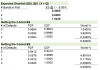
@bpdulog Here is the xls @ http://trtl.bz/es-three-bonds e.g. ,
0.0576 is a straight-up binomial PDF: Pr[X = 1 default | n = 3 bonds, p = 2%] = 2%*98%*98%*C(3,1) = 2%*98%*98%*3, because there are three combinations of one default in a 3-bond portfolio: SSD, SDS, DSS (where S=survive and D=default). Thanks,