Difference between probability density function and inverse cumulative distribution function?

[bpdulog]

What is the difference between probability density function and inverse cumulative distribution function, if any? They both look the same

 

[ShaktiRathore]

Hi,
No they are not the same.
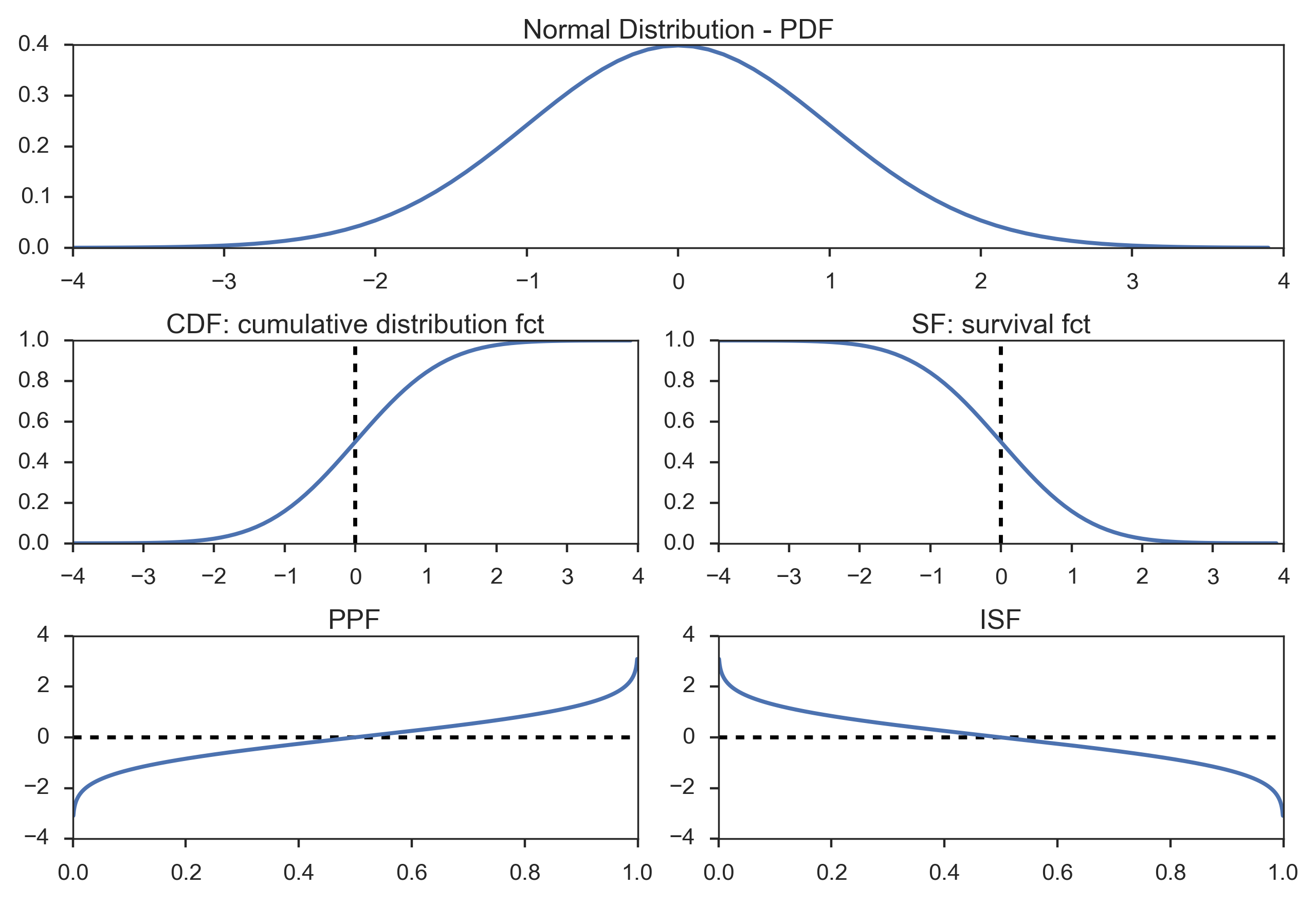
The inverse cumulative distribution function is the quantile function it gives the value of the quantile(z) at which the probability of the random variable is <=the given probability value or the cumulative probability of random variable is = the given probability value.For e.g.at 95% cumulative probability the value of quantile is z=1.645,at 99% cumulative probability z=2.33 and so on so that the plot of the values of z Vs the cumulative probability values gives the inverse cumulative distribution function ICDF. ICDF(95%)=1.645, ICDF(99%)=2.33.
Whereas probability density function P(z) gives the value of probability at a given quantile,so that when you integrate the function over a quantile range shall give the value of the cumulative distribution function,integration of P(z) over -inf to inf is=1,integration of P(z) over -inf to 1.645 is=95%,at any point z on the P(z), probability(z)=0.
thanks

 

[brian.field]

David also covers this extensively in his Study Notes for Miller. Have you read them?

 

[bpdulog]

Hi,
No they are not the same.
The inverse cumulative distribution function is the quantile function it gives the value of the quantile(z) at which the probability of the random variable is <=the given probability value or the cumulative probability of random variable is = the given probability value.For e.g.at 95% cumulative probability the value of quantile is z=1.645,at 99% cumulative probability z=2.33 and so on so that the plot of the values of z Vs the cumulative probability values gives the inverse cumulative distribution function ICDF. ICDF(95%)=1.645, ICDF(99%)=2.33.
Whereas probability density function P(z) gives the value of probability at a given quantile,so that when you integrate the function over a quantile range shall give the value of the cumulative distribution function,integration of P(z) over -inf to inf is=1,integration of P(z) over -inf to 1.645 is=95%,at any point z on the P(z), probability(z)=0.
thanks

If I understand what are you saying, in the inverse distribution the 1.645 represents 95% and less. And in the probability density function the 1.645 represents 95% only?

 

[ShaktiRathore]

Hi
in the inverse distribution the 1.645(quantile) represents 95%(cumulative probability). And in the probability density function P(x) ,when x=1.645 ,P(x) shall give the probability density at x,and we integrate the P(x) from -inf to x=1.645 to get the cumulative probability of 95%.
thanks

 

[bpdulog]

Ah ok! I think I get it now. It just 2 different ways to display a distribution of data. The top is the PDF and the PPF is basically the CDF with the axes transposed.

 

[David Harper CFA FRM]

You definitely want to understand @ShaktiRathore 's above relationship. Miller's Chapter 2 does a decent job. We don't use the continuous pdf too much. The pdf integrates to the CDF, and we're arguably more interested in the relationships around the CDF, as Shakti illustrates. For example, if probability (p) = 5.0%, then:

• p = 5% = F(q), where F(.) is the cumulative distribution function, so if we are given the probability of 5% because we want a 95% confident normal VaR, then we use the inverse CDF to retrieve the quantile:
• q = F^(-1)(p) = F^(-1)(5%) = -1.645, where F^(-1) is the inverse CDF. "Inverse" implies that F[F^(-1)(p)] = p; e.g., F[F^(-1)(5%)] = F[-1.645] = 5%, just like also F^(-1)[F(q)] = q. This is why Dowd says "VaR is just a quantile;" i.e., because -1.645 is the quantile (q) retrieved by using the inverse CDF given a probability (p) of 5%. This is an essential FRM building block. I hope that adds something.

 

[theapplecrispguy]

In Question 300.2, the final price of the bond (i.e. the value of "x") is calculated using the inverse CDF such that 5% of the distribution is less than or equal to "x". This price is calculated to be $1.842 using p=5%. My interpretation of this is that 5% of the time the bond will be priced below $1.842 and the other 95% of the time the bond will be priced above $1.842. Is this correct? The question then states that the 95% VAR is given by $5.00 (the face value of the bond) minus $1.842 (q(.05)) equals $3.158. I don't understand conceptually how the formula for 95% VAR was determined to be $5.00 - q(.05). Can you please explain what the 95% VAR ($3.158) represents in the context of the area under the cumulative distribution graph?

 

[David Harper CFA FRM]

Hi @theapplecrispguy FYI, the source Q&A (with follow on discussion) is here at https://forum.bionicturtle.com/threads/p1-t2-300-probability-functions-miller.6728/ but briefly:

• Re: "My interpretation of this is that 5% of the time the bond will be priced below $1.842 and the other 95% of the time the bond will be priced above $1.842. Is this correct?" Yes, exactly correct. The integral (anti-derivative) of the given f(x) is the CDF which is F(x) = x^3/125. When we have the CDF, it means that cumulative p = x^3/125; i.e., p is the probability that the random variable will be less than or equal to x. Because 1.842^3/125 = 5.0%, under this distribution, there is a 5.0% probability that X will be less than $1.842; and, as you say, 95.0% of the time X will be greater than $1.842 (but less than $5.00, as the function domain is $0.00 < X < 5.00). As the question is testing the associated Miller, this is really the essential point of the question ....
  
• Because the VaR part here is really simplistic. VaR is a loss relative to something. This question gives the assumption that the expected future value is $5.00 so that the VaR can be computed as a simple "worst expected loss" of $5.00 - $1.842 = $3.158; ie, because there is a 5.0% probability of the final price falling below $1.842, there is a 5.0% probability of a loss worse than $3.158. If we were not given this assumption, the proper approaches are classically either:
  • Compute the loss relative to the expected future value as the proper mean of the future distribution. In this case, as stated in the question, this relative VaR (it is called because it is relative to the expected future value) would be $3.75 - $1.842 = $1.908. I just didn't want to make the question too difficult; or,
  • Compute the loss relative to the current value, which is properly termed the absolute VaR (relative to the initial value). I don't think we have information to do that, but it would be given by discounted present value [$5.00 par] - $1.842 = absolute VaR. This shows why a good question needs to be specific about the VaR it looks for, VaR is a worst expected loss over a horizon (choice #1) with a confidence level (choice #2) relative to something (definitional #3). I hope that helps!

 

[theapplecrispguy]

Thank you David for the explanation which is very helpful. If the question had asked for the 5% VAR would the answer have been the same?

 

[David Harper CFA FRM]

Hi @theapplecrispguy Yes, but only because occasionally (or rarely) the 95.0% VaR will be represented by an author as the 0.050 VaR, treating them as the same idea. In any realistic use case, we are referring to the losses that happen in the worst 5.0% of times, the losing tail. It would not be realistic/sensible to speak of the losses that occur in the worst 95.0% of times (although mathematically it works of course). But, again, the idea is that we have a cumulative distribution function here, given by F(x) = p = x^3/125. Solving for x, we have x = (p*125)^(1/3). So for example,

• at p = 5%, x = (5%*125)^(1/3) = $1.84
• at p = 10%, x = (10%*125)^(1/3) = $2.32
  
• at p = 20%, x = (20%*125)^(1/3) = $2.92
• at p = 50%, x = (50%*125)^(1/3) = $3.97; i.e., the median
  
• at p = 95%, x = (95%*125)^(1/3) = $4.92

It's not a distribution of losses, it's a distribution of future values. We always want to be mindful of the difference, sometimes the distribution is losses. As this is future values, the risk tail is "down" at p = 5%, it is not "up" at p = 95%, so that either a 95% or 0.05 VaR would be realistically referring to the p = 5%. At the same time, there are valid usages of VaR for lower confidence levels, so we could have a 90% VaR (given by the loss of $5.00 minus $2.32) or a even an 80% VaR (given by the loss of $5.00 minus $2.92). I hope that helps!

 

[theapplecrispguy]

Thank you. Clear and much appreciated!

 

[prakashsista]

Well explained.