AIMs: Describe how a single-factor model can be used to measure conditional default probabilities given economic health. Compute the variance of the conditional default distribution and the conditional probability of default using a single-factor model. Explain the relationship between the default correlation among firms and their single-factor model beta parameters. Apply this relationship to compute one parameter from the other.
Questions:
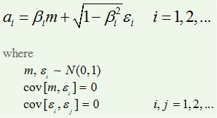
310.1. The single-factor model measures portfolio credit risk by assuming each firm (i = 1, 2, ....) has its own sensitivity to the common market factor. The sensitivity is denoted by beta(i), β(i), and the market factor is denoted by (m):

Further, as qualified above, the market and idiosyncratic shock, e(i) are random standard normal variates that are uncorrelated with one another. Assume our single-factor portfolio contains only three credits with the following betas: β(1) = 0.35, β(2) = 0.40, β(3) = 0.56. What is the implied correlation directly between credits (1) and (2), ρ(1,2)?
a. 0.140
b. 0.210
c. 0.375
d. 0.872
310.2. In Malz's single-factor model, the conditional cumulative default probability function is represented as a function of (m):

(Source: Allan Malz, Financial Risk Management: Models, History, and Institutions (Hoboken, NJ: John Wiley & Sons, 2011))
A single firm has a beta, β(i), of 0.60 and a k(i) = -1.6450. The firm's unconditional default probability is therefore 5.0%; i.e., if a(t) is ~N(0,1), the P[a(t) < k] = 5.0%. If we enter an economic downturn, such that the market factor (m) shifts to a value of -1.41, what is the economic-downturn conditional default probability?
a. 7.83%
b. 10.67%
c. 15.90%
d. 22.75%
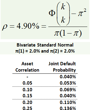
310.3. The upper panel below shows the default correlation, rho, under a single-factor credit model is 4.90% as a function of the individual default probabilities, denoted by pi. Under the simple credit model, all (both) credits have the same individual default probabilities, in this case pi = 2.0%. The joint default probability is characterizes by a bivariate standard normal distribution (joint CDF):

In the lower panel, because they require a numerical solutions, are listed the asset correlations implied by various joint default probabilities. For example, if two credits are uncorrelated, their joint PD = 2.0%*2.0% = 0.040%; if their asset correlation is 0.05, the joint PD increases to 0.053%. Given a default correlation, rho, of 4.90% what is the implied asset correlation?
a. 0.10
b. 0.15
c. 0.20
d. 0.25
Answers:
Questions:
310.1. The single-factor model measures portfolio credit risk by assuming each firm (i = 1, 2, ....) has its own sensitivity to the common market factor. The sensitivity is denoted by beta(i), β(i), and the market factor is denoted by (m):

Further, as qualified above, the market and idiosyncratic shock, e(i) are random standard normal variates that are uncorrelated with one another. Assume our single-factor portfolio contains only three credits with the following betas: β(1) = 0.35, β(2) = 0.40, β(3) = 0.56. What is the implied correlation directly between credits (1) and (2), ρ(1,2)?
a. 0.140
b. 0.210
c. 0.375
d. 0.872
310.2. In Malz's single-factor model, the conditional cumulative default probability function is represented as a function of (m):

(Source: Allan Malz, Financial Risk Management: Models, History, and Institutions (Hoboken, NJ: John Wiley & Sons, 2011))
A single firm has a beta, β(i), of 0.60 and a k(i) = -1.6450. The firm's unconditional default probability is therefore 5.0%; i.e., if a(t) is ~N(0,1), the P[a(t) < k] = 5.0%. If we enter an economic downturn, such that the market factor (m) shifts to a value of -1.41, what is the economic-downturn conditional default probability?
a. 7.83%
b. 10.67%
c. 15.90%
d. 22.75%
310.3. The upper panel below shows the default correlation, rho, under a single-factor credit model is 4.90% as a function of the individual default probabilities, denoted by pi. Under the simple credit model, all (both) credits have the same individual default probabilities, in this case pi = 2.0%. The joint default probability is characterizes by a bivariate standard normal distribution (joint CDF):

In the lower panel, because they require a numerical solutions, are listed the asset correlations implied by various joint default probabilities. For example, if two credits are uncorrelated, their joint PD = 2.0%*2.0% = 0.040%; if their asset correlation is 0.05, the joint PD increases to 0.053%. Given a default correlation, rho, of 4.90% what is the implied asset correlation?
a. 0.10
b. 0.15
c. 0.20
d. 0.25
Answers:
