Learning objectives: Describe how economic capital is derived. Explain how the credit loss distribution is modeled. Describe challenges to quantifying credit risk.
Questions:
922.1. Consider a credit portfolio that contains three positions. The exposure (EAD) of each position is $10.0 million. Further, our model assumes the shape of the loss distribution (aka, the credit risk of each exposure) is identical for each exposure, although their means vary as follows:
Which of the following is NEAREST, respectively, to the required economic capital for the second and third exposures, EC(#2) and EC(#3)?
a. $434,000 and $568,000
b. $651,000 and $852,00
c. $3.6 and $4.7 million
d. $5.9 and $7.7 million
922.2. Schroeck writes that "[t]he crucial task in estimating economic capital is, therefore, the choice of the probability distribution, because we are only interested in the tail of this distribution. Credit risks are not normally distributed but highly skewed because, as mentioned previously, the upward potential is limited to receiving at maximum the promised payments and only in very rare events to losing a lot of money. One distribution often recommended and suitable for this practical purpose is the beta distribution. This kind of distribution is especially useful in modeling a random variable that varies between 0 and c (> 0). And, in modeling credit events, losses can vary between 0 and 100%, so that c = 1. The beta distribution is extremely flexible in the shapes of the distribution it can accommodate." (Source: Gerhard Schroeck, Risk Management and Value Creation in Financial Institutions, (New York: Wiley, 2002))
In regard to the beta distribution, each of the following statements is true EXCEPT which is false?
a. The beta distribution is symmetric for all values of alpha and beta, but can only be skewed if we add a third parameter
b. The beta distribution is a continuous approximation of a binomial distribution (the sum of independent two-point distributions)
c. For high-quality portfolios--i.e., when EL(portfolio) is greater than UL(portfolio)--the beta distribution has too fat a tail and is likely to overestimate economic capital
d. For low-quality portfolios--i.e., when EL(portfolio) is less than UL(portfolio)--the beta distribution has too thin a tail and is likely to underestimate economic capital
922.3. Consider a large $20.0 million portfolio of 100 loans. In its general form, the portfolio's unexpected loss is given by:
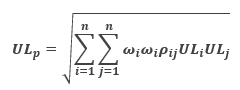
(Source: Gerhard Schroeck, Risk Management and Value Creation in Financial Institutions, (New York: Wiley, 2002))
However, each loan in this portfolio has approximately the same characteristics and size; i.e., the size of each is about $200,000. For modeling purposes, we can set the pairwise correlation coefficient to be constant ρ(i,j) = 0.160 for all i ≠ j. These assumptions greatly simplify the calculation of the portfolio's unexpected loss and each loan's contribution to portfolio risk.
In this situation, which of the following statements is TRUE?
a. A practical problem with using the general form (i.e., specifying the correlation matrix) is that default correlations are very difficult to observe
b. Under the simplifying assumptions, each loan's risk contribution (aka, unexpected loss contribution, ULC) is conveniently 16.0% of its individual unexpected loss, UL
c. If we attempted to estimate the portfolio's unexpected loss by specifying the pairwise correlation matrix of each ρ(i,j), then we would require 100! or 9.3E+157 correlation pairs
d. When estimating the portfolio's unexpected loss and its component contributions, banks prefer these analytical approaches over numerical procedures because the latter are cumbersome and prone to estimation errors
Answers here:
Questions:
922.1. Consider a credit portfolio that contains three positions. The exposure (EAD) of each position is $10.0 million. Further, our model assumes the shape of the loss distribution (aka, the credit risk of each exposure) is identical for each exposure, although their means vary as follows:
- Exposure #1 has a default probability of 2.0% and unexpected loss (UL) of $597,000
- Exposure #2 has a default probability of 4.0% and unexpected loss (UL) of $840,000
- Exposure #3 has a default probability of 6.0% and unexpected loss (UL) of $1,023,500
Which of the following is NEAREST, respectively, to the required economic capital for the second and third exposures, EC(#2) and EC(#3)?
a. $434,000 and $568,000
b. $651,000 and $852,00
c. $3.6 and $4.7 million
d. $5.9 and $7.7 million
922.2. Schroeck writes that "[t]he crucial task in estimating economic capital is, therefore, the choice of the probability distribution, because we are only interested in the tail of this distribution. Credit risks are not normally distributed but highly skewed because, as mentioned previously, the upward potential is limited to receiving at maximum the promised payments and only in very rare events to losing a lot of money. One distribution often recommended and suitable for this practical purpose is the beta distribution. This kind of distribution is especially useful in modeling a random variable that varies between 0 and c (> 0). And, in modeling credit events, losses can vary between 0 and 100%, so that c = 1. The beta distribution is extremely flexible in the shapes of the distribution it can accommodate." (Source: Gerhard Schroeck, Risk Management and Value Creation in Financial Institutions, (New York: Wiley, 2002))
In regard to the beta distribution, each of the following statements is true EXCEPT which is false?
a. The beta distribution is symmetric for all values of alpha and beta, but can only be skewed if we add a third parameter
b. The beta distribution is a continuous approximation of a binomial distribution (the sum of independent two-point distributions)
c. For high-quality portfolios--i.e., when EL(portfolio) is greater than UL(portfolio)--the beta distribution has too fat a tail and is likely to overestimate economic capital
d. For low-quality portfolios--i.e., when EL(portfolio) is less than UL(portfolio)--the beta distribution has too thin a tail and is likely to underestimate economic capital
922.3. Consider a large $20.0 million portfolio of 100 loans. In its general form, the portfolio's unexpected loss is given by:
(Source: Gerhard Schroeck, Risk Management and Value Creation in Financial Institutions, (New York: Wiley, 2002))
However, each loan in this portfolio has approximately the same characteristics and size; i.e., the size of each is about $200,000. For modeling purposes, we can set the pairwise correlation coefficient to be constant ρ(i,j) = 0.160 for all i ≠ j. These assumptions greatly simplify the calculation of the portfolio's unexpected loss and each loan's contribution to portfolio risk.
In this situation, which of the following statements is TRUE?
a. A practical problem with using the general form (i.e., specifying the correlation matrix) is that default correlations are very difficult to observe
b. Under the simplifying assumptions, each loan's risk contribution (aka, unexpected loss contribution, ULC) is conveniently 16.0% of its individual unexpected loss, UL
c. If we attempted to estimate the portfolio's unexpected loss by specifying the pairwise correlation matrix of each ρ(i,j), then we would require 100! or 9.3E+157 correlation pairs
d. When estimating the portfolio's unexpected loss and its component contributions, banks prefer these analytical approaches over numerical procedures because the latter are cumbersome and prone to estimation errors
Answers here: