Learning objectives: Explain what is meant by the statement that the mean estimator is BLUE. Describe the consistency of an estimator and explain the usefulness of this concept. Explain how the Law of Large Numbers (LLN) and Central Limit Theorem (CLT) apply to the sample mean. Estimate and interpret the skewness and kurtosis of a random variable.
Questions:
20.12.1. Barbara just received a dataset. She runs the dataset through five different regression models, where each regression model employs a different estimator for the slope. The properties of the slope estimators include the following:
a. None of the estimators are BLUE
b. Estimators A and B are both BLUE, but none of the others are BLUE
c. Estimator C might be BLUE, but none of the others are BLUE
d. Estimators D and E might both be BLUE, but none of the others are BLUE
20.12.2. In comparing and contrasting the law of large numbers (LLN) and the central limit theorem (CLT), each of the following statements is true EXCEPT which is false?
a. The LLN does not require independence but it does require normally distributed data
b. The CLT extends the LLN by requiring one additional assumption (the variance is finite)
c. LLN says that as the sample size increases (n → ∞) the Pr(X_avg = μ) approaches 100%
d. CLT says that as the sample size increases the distribution of the sample mean converges on the normal distribution N(μ, σ^2/n)
20.12.3. As an input into a Monte Carlo simulation, Derek's model generates a random standard normal deviate (aka, quantile). He conducts a test on a very small sample of ten days. His results are shown below. The first column is simply the index (1 to 10 days). The second column uses Excel's RAND() to return X which is a random continuous uniform variable (from 0 to 100%). This random probability is an input into the third column which returns a random standard normal deviate, denoted Z(i). Per Z(i) = N(-1)(X), by using Excel's NORM.S.INV(X), this performs an inverse transformation on the probability, as N(-1) is the inverse standard normal cumulative distribution function (CDF). For example, the first random uniform value is 0.21 or 21% and N(-1)(0.20) = -0.79 which means that the Pr(Z ≤ -0.79) = 21%. As a standard normal, for example, the Pr(Z ≤ 0) = 50% and Pr(Z ≤ 1.645) = 95%.
Derek wants his random series--i.e., Z(1), Z(2), ... Z(10)--to be approximately normal. However, he realizes this is a small sample so it has no right to be normal! Nevertheless, he wants to observe its first four sample moments. In regard to the first sample moment, we can see that the sample average is -0.40; the expected sample average is zero. Which of the following BEST describes the second, third, and fourth sample moments of this small sample?
a. Standard deviation is ~0.83 with positive skew and light tails
b. Standard deviation is ~0.87 with negative skew and light tails
c. Standard deviation is ~0.69 with negative skew and heavy tails
d. Standard deviation is ~1.57 with negative skew and heavy tails
Answers here:
Questions:
20.12.1. Barbara just received a dataset. She runs the dataset through five different regression models, where each regression model employs a different estimator for the slope. The properties of the slope estimators include the following:
- Estimator A is biased but has the smallest variance (3.7)
- Estimator B is linear and biased but has a small variance (4.6)
- Estimator C is linear and unbiased but has a medium variance (9.5)
- Estimator D is nonlinear and biased but is consistent and has a large variance (11.8)
- Estimator E is nonlinear and unbiased but has the largest variance (14.1)
a. None of the estimators are BLUE
b. Estimators A and B are both BLUE, but none of the others are BLUE
c. Estimator C might be BLUE, but none of the others are BLUE
d. Estimators D and E might both be BLUE, but none of the others are BLUE
20.12.2. In comparing and contrasting the law of large numbers (LLN) and the central limit theorem (CLT), each of the following statements is true EXCEPT which is false?
a. The LLN does not require independence but it does require normally distributed data
b. The CLT extends the LLN by requiring one additional assumption (the variance is finite)
c. LLN says that as the sample size increases (n → ∞) the Pr(X_avg = μ) approaches 100%
d. CLT says that as the sample size increases the distribution of the sample mean converges on the normal distribution N(μ, σ^2/n)
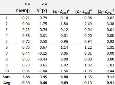
20.12.3. As an input into a Monte Carlo simulation, Derek's model generates a random standard normal deviate (aka, quantile). He conducts a test on a very small sample of ten days. His results are shown below. The first column is simply the index (1 to 10 days). The second column uses Excel's RAND() to return X which is a random continuous uniform variable (from 0 to 100%). This random probability is an input into the third column which returns a random standard normal deviate, denoted Z(i). Per Z(i) = N(-1)(X), by using Excel's NORM.S.INV(X), this performs an inverse transformation on the probability, as N(-1) is the inverse standard normal cumulative distribution function (CDF). For example, the first random uniform value is 0.21 or 21% and N(-1)(0.20) = -0.79 which means that the Pr(Z ≤ -0.79) = 21%. As a standard normal, for example, the Pr(Z ≤ 0) = 50% and Pr(Z ≤ 1.645) = 95%.
Derek wants his random series--i.e., Z(1), Z(2), ... Z(10)--to be approximately normal. However, he realizes this is a small sample so it has no right to be normal! Nevertheless, he wants to observe its first four sample moments. In regard to the first sample moment, we can see that the sample average is -0.40; the expected sample average is zero. Which of the following BEST describes the second, third, and fourth sample moments of this small sample?
a. Standard deviation is ~0.83 with positive skew and light tails
b. Standard deviation is ~0.87 with negative skew and light tails
c. Standard deviation is ~0.69 with negative skew and heavy tails
d. Standard deviation is ~1.57 with negative skew and heavy tails
Answers here:
Last edited by a moderator: