Learning objectives: Explain how asset return distributions tend to deviate from the normal distribution. Explain reasons for fat tails in a return distribution and describe their implications. Distinguish between conditional and unconditional distributions. Describe the implications of regime switching on quantifying volatility.
Questions:
803.1. Peter the Risk Analyst has collected one year (N = 250 days) of asset price data. He translates the daily prices into daily log returns; e.g., if a yesterday's price close was $5.00 and today's price close is $4.90, then the daily log return is LN(4.90/5.00) = -2.020%. His initial exploratory data analysis (EDA) of this return series includes the following observations:
a. The unconditional distribution obviously is not normal, but the unconditional distribution might fit a normal mixture distribution
b. A plausible explanation for the observed unconditional heavy tails is a distribution that is conditionally normal yet time-varying or regime-shifting
c. The zero autocovariance supports (i.e., is necessary but not sufficient to) scaling the daily standard deviation to a per annum volatility of about 23.72% = 1.50% * SQRT(250)
d. If he imposes normality by standardizing the returns per (X - µ)/σ, then Peter can expect to lower kurtosis of the returns distribution to approximately three (~3.0) and this will also shift more probability mass to the shoulders of the distribution
803.2. The daily standard deviation of a risky asset is 1.40%. If daily returns are independent, then of course we can use the square root rule (SRR) to scale into a two-day volatility given by 1.40%*SQRT(2) = 1.980%. However, if the lag-1 autocorrelation of returns is significantly positive at 0.60, then which is NEAREST to the corresponding scaled two-day volatility?
a. 1.64%
b. 1.98%
c. 2.33%
d. 2.50%
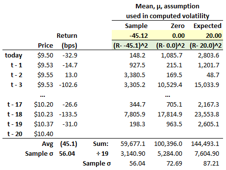
803.3. Based on daily asset prices over the last month (n = 20 days), Rebecca the Risk Analyst has calculated the daily volatility as a basic historical standard deviation (abbreviated STDEV to match Linda Allen's label for the equally weighted average of squared deviations which "is the simplest and most common way to estimate or predict future volatility"). As the exhibit below shows, however, she could not quite decide which mean, µ, to use for the sample standard deviation: the actual sample mean return was -45.12 basis points; but she has also seen zero assumed per squared returns; and finally, the expected return is actually +20.0 bps. Each produces a slightly different sample standard deviation. For example, assuming the actual sample mean produces a daily volatility of 56.04 bps which matches the Excel function STEV.S().
Which of the following statements is TRUE about Rebecca's calculations?
a. An advantage of this short 20-day window under the STDEV approach is that it minimizes the so-called ghosting effect
b. If the returns are especially heavy-tailed (ie, non-normal), this STDEV is a superior predictor to absolute standard deviation
c. If the actual 45.12 bps decline was uniquely unpredictable, it is reasonable to use the currently expected positive µ = +20 bps as the conditional mean parameter
d. While the assumption of zero mean is technically acceptable as an MLE (as opposed to unbiased) estimator of population standard deviation, it should in practice be avoided because we seek a conditional mean parameter
Answers here:
Questions:
803.1. Peter the Risk Analyst has collected one year (N = 250 days) of asset price data. He translates the daily prices into daily log returns; e.g., if a yesterday's price close was $5.00 and today's price close is $4.90, then the daily log return is LN(4.90/5.00) = -2.020%. His initial exploratory data analysis (EDA) of this return series includes the following observations:
- The lag-1 autocovariance is approximately zero
- The kurtosis of the returns distribution is about 9.50
- The daily sample standard deviation of returns is about 1.50%
a. The unconditional distribution obviously is not normal, but the unconditional distribution might fit a normal mixture distribution
b. A plausible explanation for the observed unconditional heavy tails is a distribution that is conditionally normal yet time-varying or regime-shifting
c. The zero autocovariance supports (i.e., is necessary but not sufficient to) scaling the daily standard deviation to a per annum volatility of about 23.72% = 1.50% * SQRT(250)
d. If he imposes normality by standardizing the returns per (X - µ)/σ, then Peter can expect to lower kurtosis of the returns distribution to approximately three (~3.0) and this will also shift more probability mass to the shoulders of the distribution
803.2. The daily standard deviation of a risky asset is 1.40%. If daily returns are independent, then of course we can use the square root rule (SRR) to scale into a two-day volatility given by 1.40%*SQRT(2) = 1.980%. However, if the lag-1 autocorrelation of returns is significantly positive at 0.60, then which is NEAREST to the corresponding scaled two-day volatility?
a. 1.64%
b. 1.98%
c. 2.33%
d. 2.50%
803.3. Based on daily asset prices over the last month (n = 20 days), Rebecca the Risk Analyst has calculated the daily volatility as a basic historical standard deviation (abbreviated STDEV to match Linda Allen's label for the equally weighted average of squared deviations which "is the simplest and most common way to estimate or predict future volatility"). As the exhibit below shows, however, she could not quite decide which mean, µ, to use for the sample standard deviation: the actual sample mean return was -45.12 basis points; but she has also seen zero assumed per squared returns; and finally, the expected return is actually +20.0 bps. Each produces a slightly different sample standard deviation. For example, assuming the actual sample mean produces a daily volatility of 56.04 bps which matches the Excel function STEV.S().
Which of the following statements is TRUE about Rebecca's calculations?
a. An advantage of this short 20-day window under the STDEV approach is that it minimizes the so-called ghosting effect
b. If the returns are especially heavy-tailed (ie, non-normal), this STDEV is a superior predictor to absolute standard deviation
c. If the actual 45.12 bps decline was uniquely unpredictable, it is reasonable to use the currently expected positive µ = +20 bps as the conditional mean parameter
d. While the assumption of zero mean is technically acceptable as an MLE (as opposed to unbiased) estimator of population standard deviation, it should in practice be avoided because we seek a conditional mean parameter
Answers here: