Suzanne Evans
Well-Known Member
AIMs: Describe the properties of linear combinations of normally distributed variables. Identify the key properties and parameters of the Chi-squared, Student’s t, and F-distributions.
Questions:
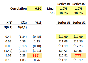
311.1. George the analyst creates a model, displayed below, which generates two series of random but correlated asset returns. Both asset prices begin at a price of $10.00 with a periodic mean return of +1.0%. Series #1 has periodic volatility of 10.0% while Series #2 has periodic volatility of 20.0%. The desired correlation of the simulated series is 0.80. Each series steps according to a discrete version of geometric Brownian motion (GBM) where price(t+1) = price (t) + price(t)*(mean + volatility*standard random normal). Two standard random normals are generated at each step, X(1) and X(2), but X(2) is transformed into correlated Y(1) with Y(1) = rho*X(1) + SQRT(1 - rho^2)*X(2), such that Y(1) informs Series #2. The first five steps are displayed below:

At the fourth step, when the Series #1 Price = $10.81, what is Y(1) and the Series #2 Price [at Step 4], both of which cells are highlighted in orange above?
a. -0.27 and $9.08
b. +0.55 and $9.85
c. +0.99 and $11.33
d. +2.06 and $12.40
311.2. Sue the risk manager is modeling a random set of 10-day asset returns. The expected annual return (drift) of the asset is 10.0% with annual return volatility of 30.0%. She assumes a discrete version of GBM such that the 10-day return = expected return*(10/250) + volatility*sqrt(10/250)*(random deviate); i.e., drift scales linearly with time and volatility scales with the square root of time. For example, assuming a normal distribution, the random uniform variable (from 0 to 1.0) on the first trial happens to be a low 0.0250. As per an inverse transformation, this corresponds to a random normal deviation of about -1.960, the modeled 10-day return = +10%*10/250 + 30%*sqrt(10/250)*(-1.960) ~= -11.360%.
Sue wants to model heavier tails, so she replaces the assumption of a normal distribution with the assumption of a student's t distribution that has only three degrees of freedom; i.e., 3 d.f. or k=3. Under this alternative assumption, given the same random uniform variable of 0.0250, what is the modeled 10-day return? (please note: this requires a student's t lookup)
a. -18.69%
b. -15.52%
c. -11.40%
d. -7.53%
311.3. In regard to the chi-squared (U^2) and F-distribution, each of the following is true EXCEPT which is false?
a. Both the chi-squared and F-distribution are non-negative and positively skewed to the right
b. The square of variable with a student's t distribution with d.f. = k has an F-distribution with 1 and k d.f.; that is, t(k)^2 ~= F(1,k)
c. The sum of two independent chi-squared variables, with respectively k1 and k2 degrees of freedom, is itself chi-squared with (k1+k2) degrees of freedom
d. The chi-squared distribution is approximated by the ratio of two independent F-distributions; i.e., U^2(k) ~ F(m,n)/F(p,q)
Answers:
Questions:
311.1. George the analyst creates a model, displayed below, which generates two series of random but correlated asset returns. Both asset prices begin at a price of $10.00 with a periodic mean return of +1.0%. Series #1 has periodic volatility of 10.0% while Series #2 has periodic volatility of 20.0%. The desired correlation of the simulated series is 0.80. Each series steps according to a discrete version of geometric Brownian motion (GBM) where price(t+1) = price (t) + price(t)*(mean + volatility*standard random normal). Two standard random normals are generated at each step, X(1) and X(2), but X(2) is transformed into correlated Y(1) with Y(1) = rho*X(1) + SQRT(1 - rho^2)*X(2), such that Y(1) informs Series #2. The first five steps are displayed below:

At the fourth step, when the Series #1 Price = $10.81, what is Y(1) and the Series #2 Price [at Step 4], both of which cells are highlighted in orange above?
a. -0.27 and $9.08
b. +0.55 and $9.85
c. +0.99 and $11.33
d. +2.06 and $12.40
311.2. Sue the risk manager is modeling a random set of 10-day asset returns. The expected annual return (drift) of the asset is 10.0% with annual return volatility of 30.0%. She assumes a discrete version of GBM such that the 10-day return = expected return*(10/250) + volatility*sqrt(10/250)*(random deviate); i.e., drift scales linearly with time and volatility scales with the square root of time. For example, assuming a normal distribution, the random uniform variable (from 0 to 1.0) on the first trial happens to be a low 0.0250. As per an inverse transformation, this corresponds to a random normal deviation of about -1.960, the modeled 10-day return = +10%*10/250 + 30%*sqrt(10/250)*(-1.960) ~= -11.360%.
Sue wants to model heavier tails, so she replaces the assumption of a normal distribution with the assumption of a student's t distribution that has only three degrees of freedom; i.e., 3 d.f. or k=3. Under this alternative assumption, given the same random uniform variable of 0.0250, what is the modeled 10-day return? (please note: this requires a student's t lookup)
a. -18.69%
b. -15.52%
c. -11.40%
d. -7.53%
311.3. In regard to the chi-squared (U^2) and F-distribution, each of the following is true EXCEPT which is false?
a. Both the chi-squared and F-distribution are non-negative and positively skewed to the right
b. The square of variable with a student's t distribution with d.f. = k has an F-distribution with 1 and k d.f.; that is, t(k)^2 ~= F(1,k)
c. The sum of two independent chi-squared variables, with respectively k1 and k2 degrees of freedom, is itself chi-squared with (k1+k2) degrees of freedom
d. The chi-squared distribution is approximated by the ratio of two independent F-distributions; i.e., U^2(k) ~ F(m,n)/F(p,q)
Answers:
