Learning objectives: Describe the models which can be estimated using linear regression and differentiate them from those which cannot. Interpret the results of an ordinary least squares (OLS) regression with a single explanatory variable. Describe the key assumptions of OLS parameter estimation. Characterize the properties of OLS estimators and their sampling distributions.
Questions:
20.16.1. Debra is an analyst at a governmental agency. Her boss asked her to investigate whether the Phillips curve applies during high-inflation regimes. To answer the question, Debra collected data from the FRED database at the St. Louis Fed (https://fred.stlouisfed.org/). The Phillips curve describes an inverse relationship between unemployment rates and inflation rates; https://en.wikipedia.org/wiki/Phillips_curve. Debra collected monthly data and she regressed the inflation rate against the unemployment rate (conditional on high-inflation regimes simply for narrative purposes). Her independent variable is the unemployment rate (FRED code: UNRATE) and here, the dependent variable is the Inflation rate (CPIAUCSL). The units are percentages not decimals; e.g., the dataset includes the month of January in 1982 when the unemployment rate was 8.90 and the inflation rate was 6.38. Her regression results are presented below.

Debra wants to know if an inverse relationship is observed. Which of the following statements about the regression is TRUE?
a. The regression is not useful because the intercept is too far away from (different than) zero
b. The pattern of the standard errors, t-statistics, and p-values suggest there is a violation in some assumption(s) of the classical linear regression model (CLRM)
c. There is an inverse relationship because, for each unit increase in the unemployment rate (i.e., +1.0%), the inflation rate is expected to decrease on average by 1.10%
d. There is not an inverse relationship because, for each unit increase in the unemployment rate (i.e., +1.0%), the inflation rate is expected to increase on average by 5.60%
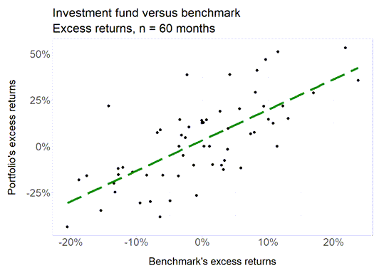
20.16.2. Peter is an analyst who is evaluating an investment fund whose managers claim has outperformed their benchmark. He collected monthly returns for the last five years; i.e., the sample size is excess return pairs over n = 60 months. He plots excess returns, which are defined as the returns in excess of the riskfree rate; ie., an excess return equals the gross return minus the riskfree rate. The scatterplot is displayed below:

The correlation coefficient is 0.708. In regard to the univariate data, the standard deviation of the portfolio's returns is 22.84% and the standard deviation of the benchmark's returns is 9.79%. The average excess return of the benchmark was -0.37% and the average excess return of the portfolio was 2.61%. Each of the following statements is true EXCEPT which is false?
a. The slope of the regression line is approximately 1.65 and the intercept is approximately 3.22%
b. Visual inspection confirms the error variance is not constant and we can, therefore, assert the presence of heteroskedastic shocks
c. This regression line passes through the coordinates of averages, (μ_x, μ_y) = (-0.37%, +2.61%), although this is not an actual pairwise observation
d. This model appears to at least meet the three essential restrictions of a linear regression model including linearity in the coefficients (aka, parameters)
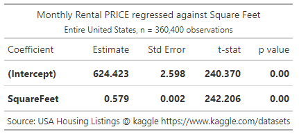
20.16.3. Sally works at a real estate firm and was asked by her client to quantify the relationship between rental size (in square feet) and rental price. She explained to her client that the relationship is multivariate but, given that caveat, she offered to perform a linear regression with a single explanatory variable. She retrieved a massive dataset (n = 360,400 observations and includes rentals across the United States) and regressed monthly rental price (aka, the explained variable) against rental size as measured by square feet. To illustrate the units, one of data points in the dataset is (y = $1,200 per month, X = 1,000 feet^2). The results are displayed below.

In regard to Sally's interpretation of these regression results (above), each of the following statements is true EXCEPT which is false?
a. The model predicts a rent of $2,072 for a size of 1,800 feet^2
b. The mean residual is zero; i.e., the average of 360,400 residuals is zero
c. Both the intercept and slope coefficients are significant; aka, significantly different than zero
d. Each increase in the rental size of 100 feet^2 is associated with an average increase of $57.90 in monthly rent
Answers here:
Questions:
20.16.1. Debra is an analyst at a governmental agency. Her boss asked her to investigate whether the Phillips curve applies during high-inflation regimes. To answer the question, Debra collected data from the FRED database at the St. Louis Fed (https://fred.stlouisfed.org/). The Phillips curve describes an inverse relationship between unemployment rates and inflation rates; https://en.wikipedia.org/wiki/Phillips_curve. Debra collected monthly data and she regressed the inflation rate against the unemployment rate (conditional on high-inflation regimes simply for narrative purposes). Her independent variable is the unemployment rate (FRED code: UNRATE) and here, the dependent variable is the Inflation rate (CPIAUCSL). The units are percentages not decimals; e.g., the dataset includes the month of January in 1982 when the unemployment rate was 8.90 and the inflation rate was 6.38. Her regression results are presented below.

Debra wants to know if an inverse relationship is observed. Which of the following statements about the regression is TRUE?
a. The regression is not useful because the intercept is too far away from (different than) zero
b. The pattern of the standard errors, t-statistics, and p-values suggest there is a violation in some assumption(s) of the classical linear regression model (CLRM)
c. There is an inverse relationship because, for each unit increase in the unemployment rate (i.e., +1.0%), the inflation rate is expected to decrease on average by 1.10%
d. There is not an inverse relationship because, for each unit increase in the unemployment rate (i.e., +1.0%), the inflation rate is expected to increase on average by 5.60%
20.16.2. Peter is an analyst who is evaluating an investment fund whose managers claim has outperformed their benchmark. He collected monthly returns for the last five years; i.e., the sample size is excess return pairs over n = 60 months. He plots excess returns, which are defined as the returns in excess of the riskfree rate; ie., an excess return equals the gross return minus the riskfree rate. The scatterplot is displayed below:

The correlation coefficient is 0.708. In regard to the univariate data, the standard deviation of the portfolio's returns is 22.84% and the standard deviation of the benchmark's returns is 9.79%. The average excess return of the benchmark was -0.37% and the average excess return of the portfolio was 2.61%. Each of the following statements is true EXCEPT which is false?
a. The slope of the regression line is approximately 1.65 and the intercept is approximately 3.22%
b. Visual inspection confirms the error variance is not constant and we can, therefore, assert the presence of heteroskedastic shocks
c. This regression line passes through the coordinates of averages, (μ_x, μ_y) = (-0.37%, +2.61%), although this is not an actual pairwise observation
d. This model appears to at least meet the three essential restrictions of a linear regression model including linearity in the coefficients (aka, parameters)
20.16.3. Sally works at a real estate firm and was asked by her client to quantify the relationship between rental size (in square feet) and rental price. She explained to her client that the relationship is multivariate but, given that caveat, she offered to perform a linear regression with a single explanatory variable. She retrieved a massive dataset (n = 360,400 observations and includes rentals across the United States) and regressed monthly rental price (aka, the explained variable) against rental size as measured by square feet. To illustrate the units, one of data points in the dataset is (y = $1,200 per month, X = 1,000 feet^2). The results are displayed below.

In regard to Sally's interpretation of these regression results (above), each of the following statements is true EXCEPT which is false?
a. The model predicts a rent of $2,072 for a size of 1,800 feet^2
b. The mean residual is zero; i.e., the average of 360,400 residuals is zero
c. Both the intercept and slope coefficients are significant; aka, significantly different than zero
d. Each increase in the rental size of 100 feet^2 is associated with an average increase of $57.90 in monthly rent
Answers here:
Last edited by a moderator:
